Chapter 4 Case Study: Studying Quotes
After having studied trades, we now move to studying quotes extensively. An order can be subject to the action insert, update or remove.
Limit Order Insertion
An order insertion is always the first step in the lifecycle of the order.
A limit order indicates the placement of an order that only trades at a price that is not worse than its predetermined limit price specified by the trader.
As the price of the limit order is not necessarily offered on the opposite of the market, a limit order faces execution risk.
If no trader is willing to cover the opposite of the trade at the predetermined price, the limit order remains in the market.
All limit orders in the order book are queued based on price and time priority.
The larger the distance of the limit price and the midpoint, the higher the execution risk, or the time until the order is filled.
To avoid large order durations, the trader places limit orders with a smaller distance to the inside.
Limit orders at the best bid or offer are called at the market.
Accordingly, limit orders with prices worse (better) than the current best quotes are called behind (in) the market.
The limit order is removed from the order book, once it is filled completely or until the trader decides to remove it from the book unfilled.
Limit Order Update
Subsequent to its insertion, the order can be updated.
An update happens if the trader manually adjusts the limit price or overall size of the order, or the order is partially filled.
A partial fill in the data will be flagged as action UPDATE while simultaneously indicating an execution of the order and adjustment of the corresponding order size.
Limit Order Removal
The final stage in the order lifecycle is its removal. An order might be removed if the trader manually decided to cancel the order (partially) unfilled, or if the order is fully filled.
A limit order is filled when the market price reaches the specified limit price set by the order. The process of filling a limit order depends on whether it’s a buy limit order or a sell limit order:
When a limit order is filled by a market order, it means that another market participant (usually a trader or investor) has placed a market order that matches the conditions of the limit order. Here’s how it typically works:
If you’ve placed a sell limit order and the market price rises to or above your specified limit price, your order will be filled by a market order placed by another participant who is willing to buy at that price or higher. Again, market orders are executed immediately at the best available price, so when your sell limit order matches the conditions of someone’s buy market order, your order will be filled at the prevailing market price.

4.1 Data Manipulation
The quotes dataframe contains incremental order book data. That means, each row depicts a single message. A message refers to the action happing to a specific order within the book and can either capture the event of an order insertion, an order update or an order removal. By using a unique identifier for each inserted limit order, an order can be traced from its initial insertion into the limit order book until its final removal, either through execution against a trade or another order or through the command to remove the order. Whenever a change to the prevailing quotes occurs, a new row is added to the data that captures the order book action.
The data is reported in nanosecond granularity.
We start by loading and investigation the dataframe containing quotes data and remove columns which are redundant for our analysis to allow for faster computation. To avoid distortions due to intraday auctions, we remove all orders that are inserted before 8.40, during 11.55 and 12.05 and after 16.20.
Index(['side', 'price', 'size', 'order_id', 'event_timestamp', 'lob_action',
       'old_price', 'old_size', 'old_order_id', 'order_executed',
       'execution_price', 'execution_size', 'price_level', 'old_price_level',
       'best_ask_price', 'best_ask_size', 'total_ask_size', 'best_bid_price',
       'best_bid_size', 'total_bid_size', 'is_new_best_price',
       'is_new_best_size', 'original_order_id', 'trade_id', 'size_ahead',
       'orders_ahead', 'market_state'],
      dtype='object')
The record of each incremental order book update contains the following information: order_id, price, size, order side, market_state, action type (insert, update, removal), and the general state of the order book at the time of the trade (best bid, best ask (bid) size and best ask (bid) price, number of orders ahead). To get a first idea of the data, we investigate the first 20 rows of the dataframe.
Our data allows to trace a single order by investigating the order_id throughout the evolution of the order book. Notice that the existence of the column old_order_id indicates that the initial order_id generated upon order insertion might be subject to changes as the order moves through the book.
4.2 Joining
Joining describes the process of combining the rows of two dataframes based on identical values in a column that is available in both of the dataframes. We therefore briefly review the most common ways to join two dataframes.
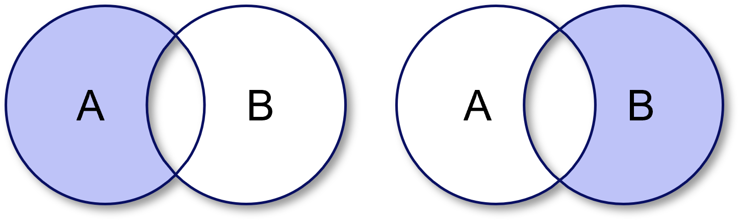
A full left join uses all rows from the table specified first in the query, hence the name left join, regardless of whether a matching row in the right table can be found. If the row cannot be matched, NaN values are induced for the right table. In essence, a left join ensures that all records from the left table are included in the resulting dataframe, while a right join ensures that all records from the right table are included in the resulting dataframe.
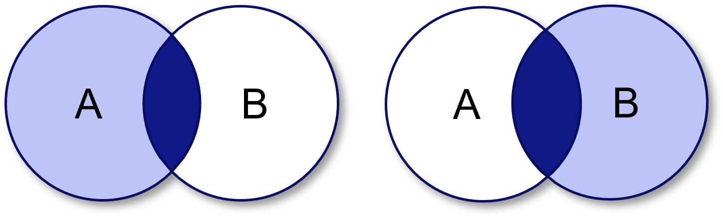
An outer join is a database operation that is based on the concept of a one-sided join but only returns all rows which could not be matched to the other dataframe. This kind of join is particularly well-suited for investigating differences between two dataframes.
Joining Order Insertions and Order Updates
To allow for easier comprehension of underlying order book dynamics and faster computation of order book metrics, we aim to structure our dataframe in a way, that we left join all order updates and removals onto all order insertions.
We receive a dataframe that contains all order insertions stacked above one another, with the corresponding order updates and removals at the right side of the dataframe. This means that each row is a unique combination of an insertion and one subsequent order book update or removal for the inital order insertion. Order ids that occur only once in the dataframe, are not updates - they are only removed after their initial insertion. Order ids that occur multiple times in the dataframe are updated before their final removal.
We can investigate the first 100 values of the dataframe:
Such a structure allows us to easily compute the time difference between the initial order insertion and the subsequent order update or removal.
4.3 Bucketing
Data bucketing, also known as data binning or discretization, is a fundamental technique in data preprocessing and later data analysis. It involves dividing a continuous dataset into smaller, distinct groups - commonly known as “buckets” - based on specific criteria or value ranges. Bucketing therefore reduces the complexity of the dataset by decreasing the number of unique values an attribute can take. Such an approach is especially relevant when it comes to uncovering patterns and trends within the data.
One economically logical way of bucketing quotes is to bucket observations by size. The size of an inserted order is a discrete variable that can take a lot of values \(Q = \{1,2,...,10000\}\). As this realization is way too granular for further analysis, we classify the order sizes more generally. Therefore, we design an arbitrary list of cutoff values for each bucket and corresponding bucket labels which correspond to the upper limits of each interval.
4.4 Grouping
Data grouping is the process of organizing and aggregating data based on common characteristics or attributes. It involves the grouping rows of data that hold identical values in one or more columns and requires a specification of an aggregation function. The aggregation function, such as sum, count, average, min, max, std and others, is then used to calculate summary statistics per group. By convention, grouping makes most sense to apply with discrete values. It is therefore oftentimes used in conjunction with bucketing or discretization of data.
We apply the grouping to all numeric columns of the dataframe.
# Filter for numeric columns
import numpy as np
numerics = list(quotes.select_dtypes(include=np.number).columns)

# Group by size bucket
quotes.groupby("size_bucket")[numerics].mean()
We can use multiple attributes for grouping as well.
4.5 Market Quality
Measuring market quality involves assessing how easily assets can be bought or sold without causing significant price movements. Typical measures to gauge the market quality are spreads, market depth, market volatility, price impacts. We go through the computation and interpretation of some metrics in the following sections.
We work with the discretized data and compute the relevant metrics for every interval:
def discretize(quotes, freq):
  # Convert timestamp to datetime column
  quotes["event_timestamp"] = pd.to_datetime(quotes["event_timestamp"])

  # Specify modes of aggregation
  agg_dict = {"price":["mean", "min", "max"],
              "size":["mean", "sum"],
              "best_ask_price":["mean", "min", "max"],
              "best_bid_price":["mean", "min", "max"],
              "best_ask_size":"mean",
              "best_bid_size":"mean",
              "order_id":"count"}

  # Discretize
  quotes_discretized = quotes.resample(freq, on="event_timestamp")\
                             .agg(agg_dict)\
                             .reset_index()

  return quotes_discretized


quotes_discretized = discretize(quotes, "5min")
4.5.1 Spread
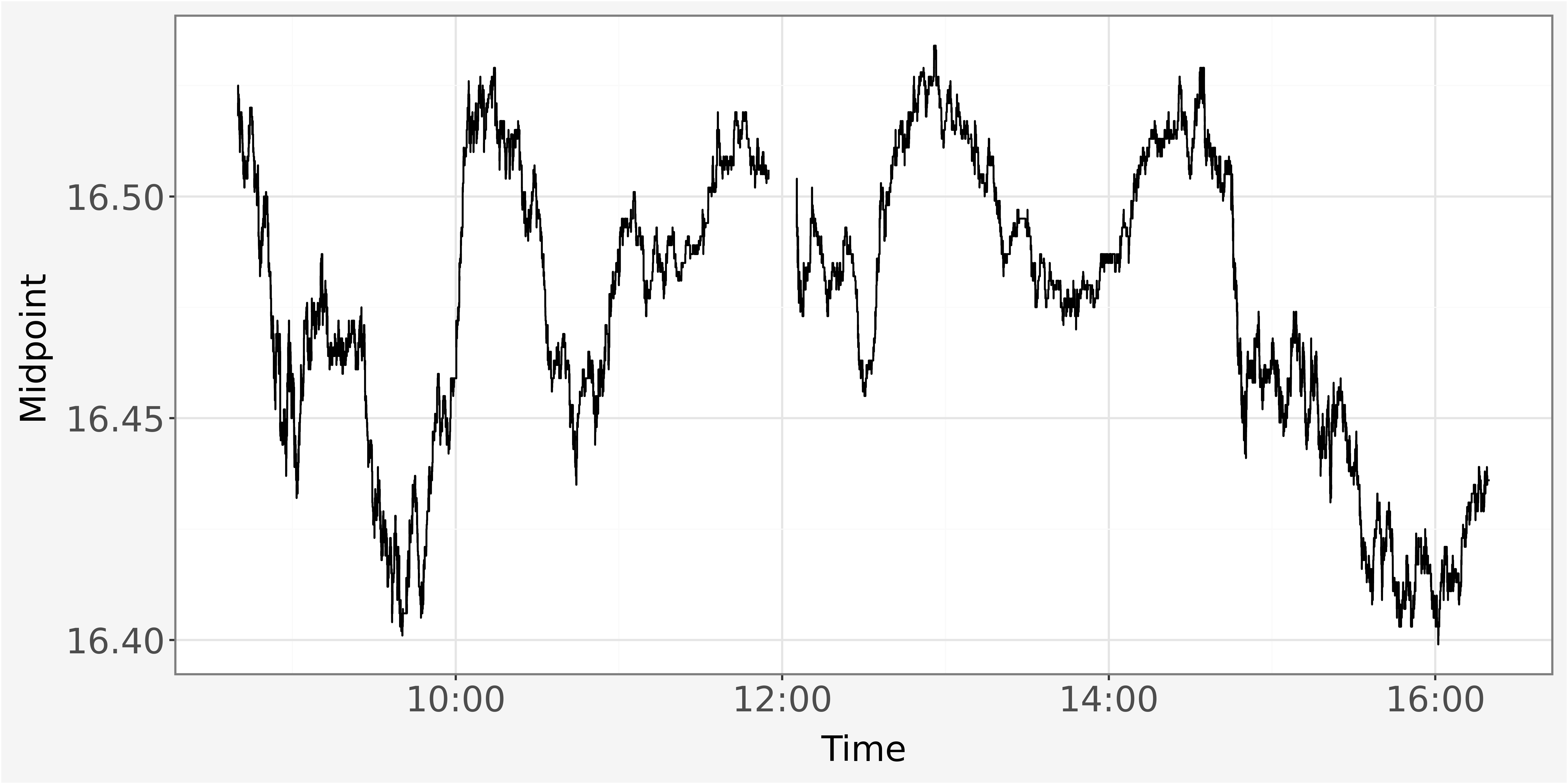
We plot the evolution of the best bid and best ask prices by investigating the shifts in the midpoint \(MID_t\) throughout the trading day to infer about an potential liquidity increase or decrease. The midpoint is calculated as average of best bid \(P_t^b\) and best ask \(P_t^a\) price:
\(MID_t=(P_t^a + P_t^b ) \times 0.5\)
The difference between best bid and best ask price is ultimately known as the quoted spread \(QS_t\) and calculated as difference between best ask price and best bid price.
\(QS_t=P_t^a - P_t^b\)
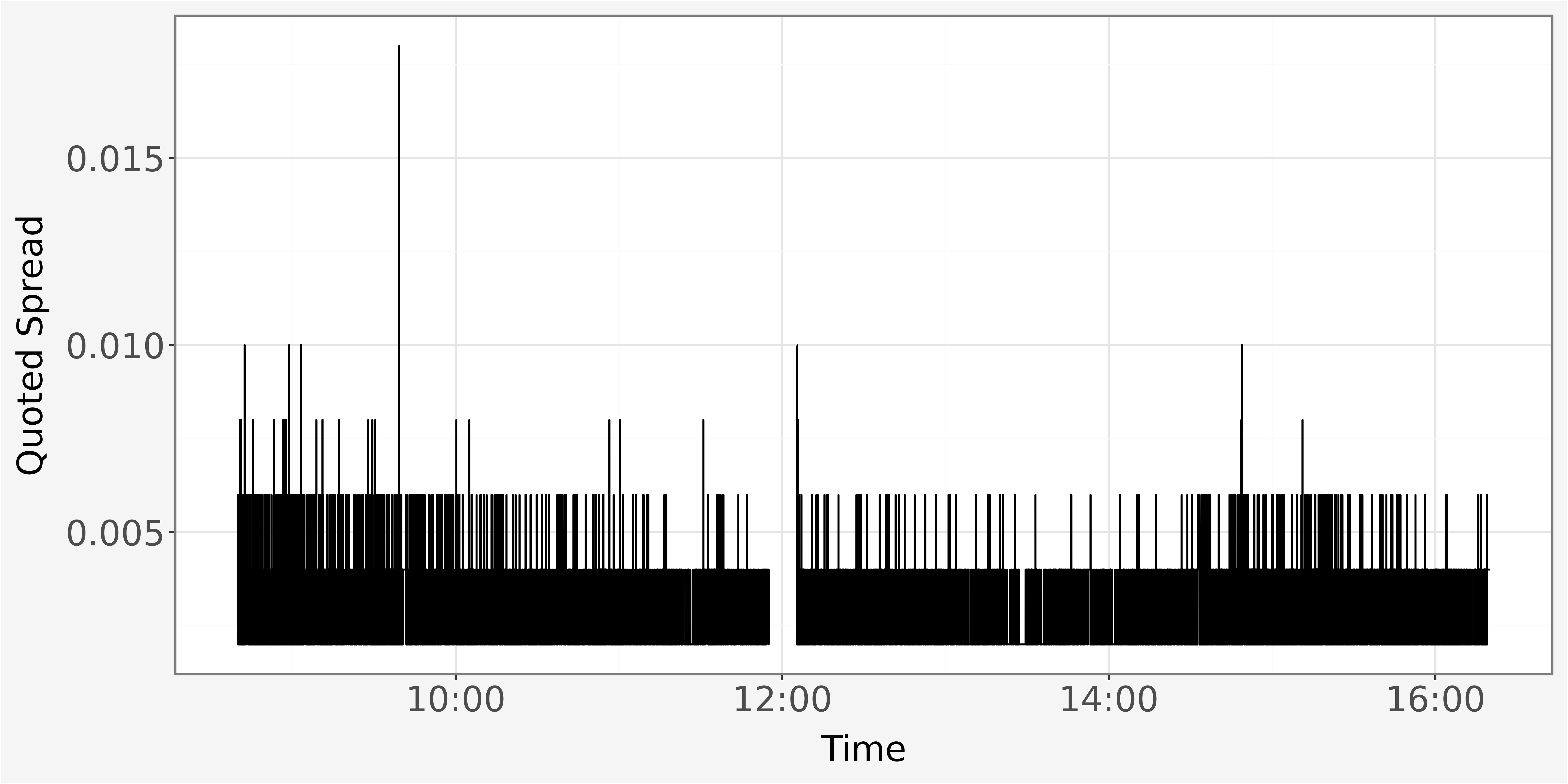
We observe the quoted spread as discrete value. It takes values such as \(0.002, 0.004\) or \(0.006\). This is the because the price levels available on an exchange are set in fixed increments, also commonly known as “Ticks”. Those fixed increments determine the minimum price movements which is allowed in the market. For our sample, we observe a minimum price movement of \(0.002\) Euros or Ticks, equivalent to \(0.2\) Cent.
# Investigate different values of the bid price
quotes.best_bid_price.sort_values().unique().tolist()[0:10]
[16.398, 16.4, 16.402, 16.404, 16.406, 16.408, 16.41, 16.412, 16.414, 16.416]Because the bid and ask prices are based on these fixed price increments, the quoted spread also appears in discrete values and cannot be smaller than the minimum tick size.
4.5.2 Order Imbalance
The measure of order imbalance captures the disparity between the number of buy orders and sell orders at a given time in the order book. It can either be computed based on pure quantities or volume available. Order imbalances can be computed for different levels of the order book \(l = \{1,2,...,L\}\). The maximum level for which the order imbalance can be computed is usually determined by information available in the dataset. In general, the order imbalance up to level \(l\) can be computed based on pure order quantities as
\(IMB_t^{quantity}=\frac{\sum_{i=1}^l Q_{t,l}^{a} - Q_{t,l}^{b}}{\sum_{i=1}^l Q_t^{a} + Q_{t,l}^{b}}\)
Alternatively a computation based on order volume can be computed, as:
\(IMB_t^{volume}=\frac{\sum_{i=1}^l (Q_{t,l}^{a} \times P_{t,l}^{a}) - (Q_{t,l}^{b} \times P_{t,l}^{b})}{\sum_{i=1}^l (Q_t^{a} \times P_{t,l}^{a}) + (Q_{t,l}^{b} \times P_{t,l}^{b})}\)
The order imbalance therefore takes values \(imb_t \in [-1,1]\). Negative value indicates buy pressure as the quantities on the bid side outweigh the quantities on the ask side while a positive value indicates sell pressure as the quantities on the ask side outweigh the quantities on the bid side.
As our data only provides information about the inside market (level one) we can only compute imbalances for the first level in the data. Technically, we could use the quotes dataframe to reconstruct the limit order book at any given point in time and then calculate imbalances at different levels. However, as this is rather computationally intense, we refrain from modelling imbalances on higher levels.
def get_imbalance(data):

  data["imbalance_quantity"] = (data["best_ask_size_mean"] - data["best_bid_size_mean"]) / (data["best_ask_size_mean"] + data["best_bid_size_mean"])
  data["imbalance_volume"] = (data["best_ask_size_mean"] * data["best_ask_price_mean"] - data["best_bid_size_mean"] * data["best_bid_price_mean"]) / (data["best_ask_size_mean"] * data["best_ask_price_mean"] + data["best_bid_size_mean"] * data["best_bid_price_mean"])

  return data
4.5.3 Volatility
In previous sections, volatility has been as sum of squared returns over different time intervals, we now introduce another definition to capture volatility. We now measure volatility as difference between the highest and lowest price level within all observations of an intraday interval which contains \(n\) observations. The prices within the interval can therefore be formalized as \(p_i = {p_1, p_2, ..., p_n}\). Formally, we model the volatility as:
\(\sigma_t^2 = \frac{max(p_i) - min(p_i)}{\frac{1}{n}\sum_\gamma^n p_\gamma}\)
Notice that volatility in such a way can be computed for nearly all metrics within our sample. We therefore design our function for the computation of volatility with another keyword argument that requires the user to specify a column which should be used for the computation.
Our pythonic implementation reads as:
4.6 Exercise
Computation| (0) | Read the data from the corresponding .csv files and filter for all order book events happening during hours of CONTINUOUS TRADING. |
| (1) | When do you find the value order_id in the order book to be missing? How does this impact the results using the matching algorithm proposed in section Joining? |
| (3) | Identify all orders that have been inserted more than once. Sort the dataframe by timestamp and remove the first occurrence of the double inserted orders. |
| (4) | Calculate the average duration between an order insertion and a consecutive order action (update or remove). Present the results grouped by the type of consecutive order action and insertion size. |
| (5) | Filter the dataframe to contain only orders which have been inserted and removed on the same day. |
| (6) | Compute the intraday Order-to-trade ratio, as \(OTR_i = \frac{Number of messages_i}{Number of trades_i}\), for each 5-minute interval. The Number of messages relates to all order book activities (insertions + updates + removes), the number of trades relates to all order removals due to the order being filled (lob_action == REMOVE and order_executed == True). |
| (7) | Calculate the quoted spread on the discretized and the event-time dataframe. Plot both spreads throughout the trading day. Do you observe any difference in the spread’s pattern? Why does this difference occur?. |
| (8) | Build a function that discretizes a given dataframe of quotes and takes the discretization interval as input parameter. Run a loop over a the function that discretizes the quotes data on 1-minute, 5-minute, 10-minute, 30-minute and 60-minute intervals. |
| (9) | Plot the average and total number of order insertions per discretized interval throughout the trading day for different interval lengths (1-minute, 5-minute, 10-minutes, 30-minutes and 60-minutes) using the previously generated function. |