Chapter 3 Case Study: Studying Trades
After having learned about basic coding concepts, we are well equipped to work on a first dataset. Supporting literature for this section is Econometrics of Financial High-Frequency Data - Nikolaus Hautsch.
Our dataset contains trade and quote data. Trade data is associated with information on individual trades consisting of a trade timestamp, the trade execution price and trade execution size, usually expressed in number of shares. Quote data contains information about the limit order book, event timestamps, best bid and ask quotes, and market depth. Additional to the limit order book data, we utilize message data on all limit order activities. Such type of data provides full information on all limit order activities throughout the trading day. A message can be generated by an order insertions, an order update, a (partial) fill and order cancellation. Data on the message traffic throughout the trading day allows to trace a single order through the order book and reconstruct its lifecycle. It additionally allows to reproduce the entire order flow, and therefore the limit order book, at any given point in time.
The contents of the section are specially tailored to financial high frequency data. However, most concepts are equally transferable to data with any other domain. Generally, this section evolves around the process of data exploration, cleaning and discretization. Data exploration defines as the process of analyzing and understanding a dataset to gain first insights and generate knowledge about it without a (specific) research question (yet). During the process of data exploration, you may perform tasks such as visualizing the data, generating new variables, summarizing key metrics, identifying missing values and outliers, and assessing the quality of the data.
Throughout the remainder of this book, we examine the empirical properties of ultra high-frequency data by using Telekom, traded at XETRA on the 21-02-2020. This chapter focussed on the analysis and statistical properties of trade data.
3.1 Preprocessing
Data preprocessing covers the process of transforming raw data into a form suitable for an extensive analysis and final model development. The step of data preprocessing proves vital as empirical data is often incomplete, inconsistent, or contains anomalies. Leaving those inconsistencies unrecognized is likely to result in inaccurate, biased or spurious results. Dependent on how confident you are in the quality of your dataset, you might want (or need) to run the following checks for data quality. Which steps are applicable and necessary are, of course, conditional on your own dataset and research question.
Our trades dataframe contains information on the trades’ timestamp, its execution price, execution size, the market state the trade was executed and the type of the trade. We investigate the available metrics within our dataframe:
Index(['trade_id', 'trade_timestamp', 'publication_timestamp',
       'aggressor_side', 'price', 'execution_size', 'market_state',
       'trade_type'],
      dtype='object')
More detailed information about the variables available in the dataset can be found in the corresponding data dictionary. In order to (later) perform manipulations on our datetime columns, we transform them into the corresponding datetime format.
trade_id                   int64
trade_timestamp           object
publication_timestamp     object
aggressor_side            object
price                    float64
execution_size             int64
market_state              object
trade_type                object
dtype: objectData Cleaning
Data cleaning is the process of identifying and correcting or removing errors, inconsistencies, and inaccuracies in a dataset. It might be necessary to run statistical tests on the data to identify outliers and anomalies which look like they have been generated by a different data generating process. Additionally, having domain knowledge helps you to identify obvious erroneous data within the dataset (this does requires READING about your topic!). When investigating order book data, e.g., a negative bid-ask spread would be something to investigate more closely.
Prior to any exploratory work, we start by filtering our trade data. Commonly, high frequency data is cleaned by (1) removing observations which are incorrect, delayed or subsequently corrected, (2) filtering for regular trading hours, (3) removing zero, negative prices or sizes.
We start by cleaning our trades dataframe and apply vertical filtering for the trading condition LIT and only keep those trades executed within continuous trading sessions.
trade_type = "LIT"
market_state = "CONTINUOUS_TRADING"

trades = trades[(trades["trade_type"] == trade_type) & \
                (trades["market_state"] == market_state)].reset_index(drop=True)
Data Transformation
Data transformation refers to the process of converting data from one format, structure, or representation to another format. It involves the manipulation and changing of data in order to make it more suitable for a particular analysis. Within the process, (1) new features from existing data are created, such as calculating ratios, differences, or percentages between different variables, (2) categorical data is encoded to numerical values, such as assigning numeric codes to represent different categories (review section [Python Basics]) or (3) multiple datapoints are aggregate into a single datapoint.
We furthermore extend our available metrics by computing the traded volume per trade. We do so by multiplying execution size and execution price.
3.2 Descriptives
Descriptive statistics are numerical and graphical methods used to summarize and describe the characteristics of a dataset. These statistics provide a concise summary of the main features of the data, allowing for easier interpretation and understanding. Descriptive statistics are commonly used in exploratory data analysis to gain insights into the distribution, central tendency, dispersion, and shape of the data.
We can compute some initial measures of distribution for the trades using the describe.
           price  execution_size
count 15757.0000      15757.0000
mean     16.4768        639.7228
std       0.0428        844.9231
min      16.4000          1.0000
25%      16.4480        238.0000
50%      16.4760        500.0000
75%      16.5060        866.0000
max 16.6340 35246.0000While the price shows on overall rather low dispersion, the execution size is highly dispersed and skewed to the right. This is because we observe few, but very large trades. We can use the initial descriptives to infer about potential outliers by looking looking at the values at the tails of the distribution followed by a more extensive analysis of our dataset.
# Compute standard deviation
std_quantity = np.nanstd(trades.execution_size).round(4)
# Compute mean
mean_quantity = np.nanmean(trades.execution_size).round(4)
# Compute median
median_quantity = np.nanmedian(trades.execution_size).round(4)

volume_mean = trades.drop("trade_id", axis=1).describe()["execution_size"]["mean"]
We summarize the following stylized facts about high-frequency data: Virtually, all high-frequency trading metrics are strongly serially correlated. This finding remains true for data discretized on time, causing equi-distant observations, discretized on events, causing irregularly spaced financial durations. Many metrics take only positive values while howing a high degree of skewness. Nearly all metrics are subject to strong intraday periodicities.
3.3 Visualization
Data visualization aims to reduce the degree of abstraction by illustrating data in an at least two-dimensional way. It is a powerful tool for exploring and communicating complex datasets in a clear and concise way and is particularily useful when working with large amounts of data. By using visual elements like charts, graphs, maps, and infographics, data visualization can make patterns, trends, seasonalities, anomalies and correlations within the data more easily recognizable.
There are several packages to visualize data, such as matplotlib, seaborn, plotly or ggplot. Within this document, we use Plotnine, which is available for both, Python and R, for visualization purposes.
In order to allow proper visualization of the data it is necessary to identify relevant metrics that require plotting, as well as the selection of an appropriate visual. We start by plotting trade price and volume throughout the day discretized on a one-minute time interval and investigate the traded quantities per trade within our dataset.
size_mean = trades.drop("trade_id", axis=1)\
                  .describe()["execution_size"]["mean"]

volume_mean = trades.drop("trade_id", axis=1)\
                    .describe()["volume"]["mean"]
<Figure Size: (1000 x 500)>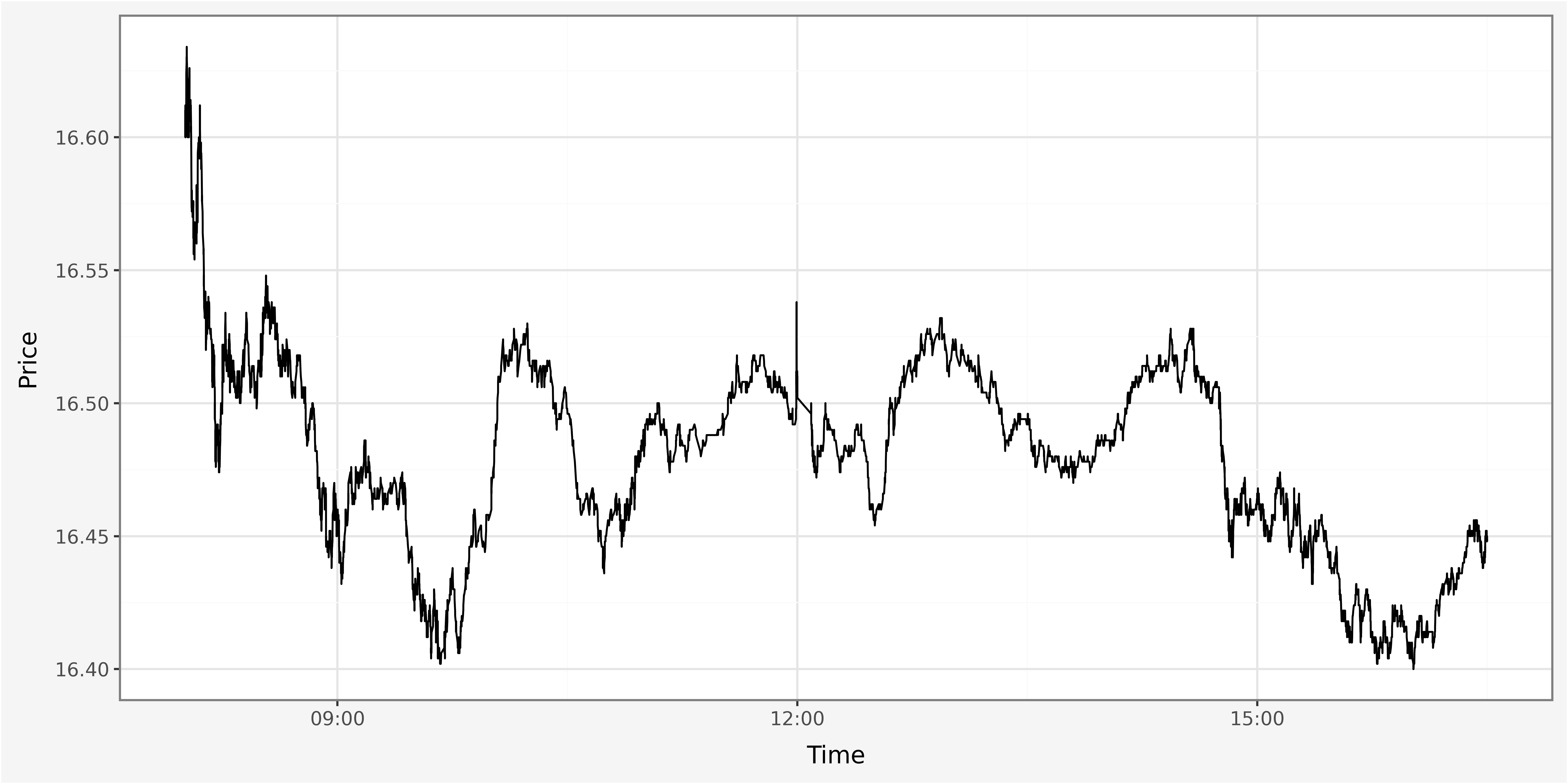
<Figure Size: (1000 x 500)>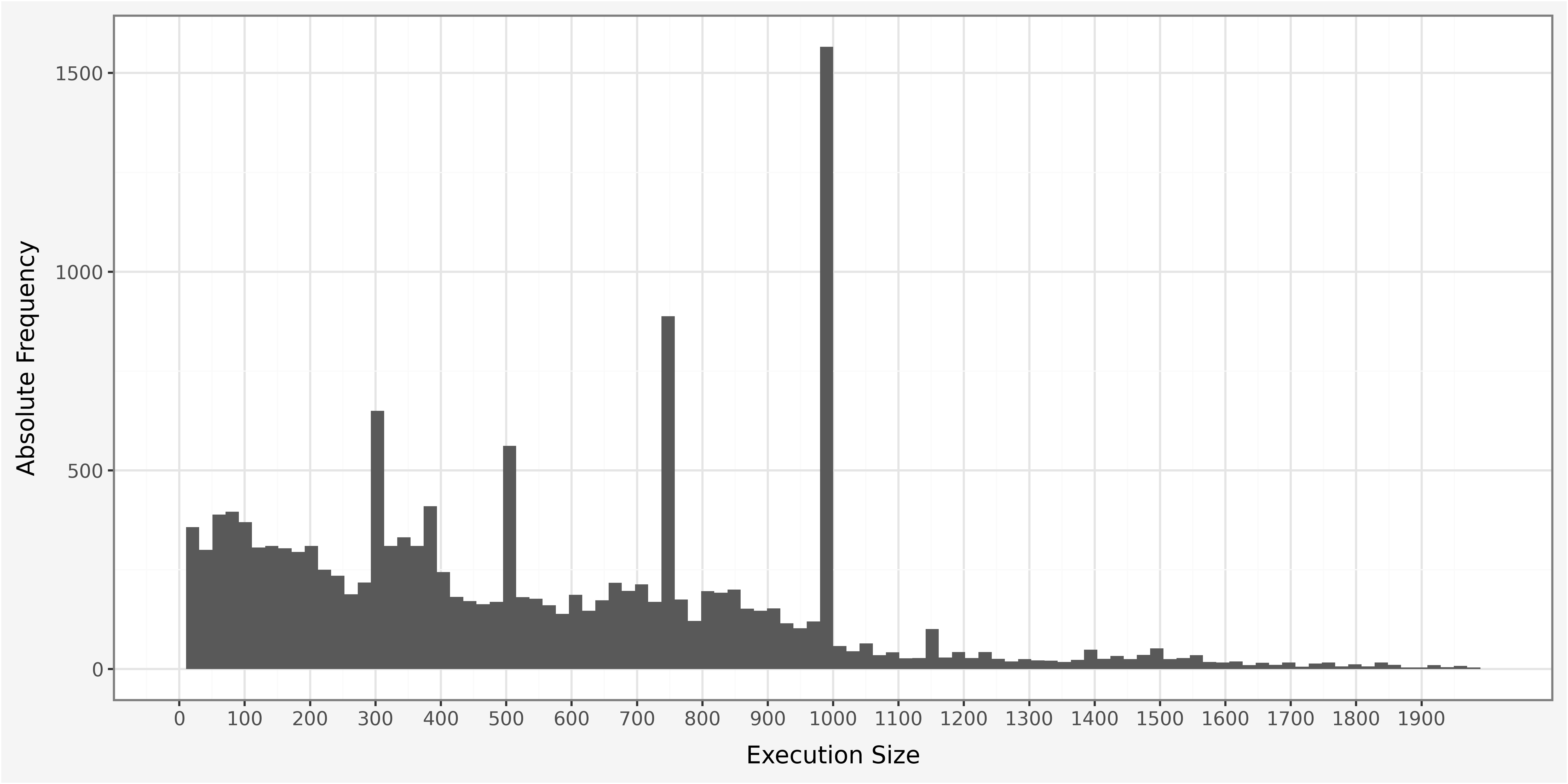
The histogram provides strong visual evidence for the concentration of probability mass around round numbers, reflecting the stylized phenomenon of traders’ preferring to trade in round lots.
3.4 Discretization
When working with tick-level data, our data is not evenly spaced. That means, events occur in continuous time. Oftentimes, we aggregate the data to lower frequencies and an evenly spaced timegrid for further analysis. There are three major reasons of doing this. First, the discretization allows to construct economically relevant variables (volume per minute, realized volatility). Second, market microstructural effects that mainly cause statistical noise are reduced (bid-ask bounce). Third, it serves to reduce the amount of data while keeping information loss to a minimum. This is especially relevant when dealing with a large time series of (cross-sectional) data. Evaluating market activity over equi-distant time intervals has the advantage that the data are by construction synchronized which eases a cross-sectional comparision over multiple assets.
Generally, we can either aggregate by event or by time. An aggregation by event indicates to aggregate all observations between two consecutive events occuring. Likewise, an aggregation by time indicates to aggregate all observations between two consecutive events in calender time.
We use a dictionary to define how every column in the dataframe should be aggregated. We decide to discretize the dataframe to one-minute time intervals, however the function allows to a specturm of broader (months) or even finer (miliseconds) time intervals for data discretization. After having discretized the data, our dataframe has two column levels. This is due to the aggregation using a dictionary. To flatten the dataframe (this means, to bring the column back to single level columns), we iterate over the columns in the dataframe and concat the first and second level of the column.
# Discretize Data to minutes
trades_discretized = trades.set_index("trade_timestamp")\
                           .resample("1min")\
                           .agg({"trade_id": "count",
                                 "price":"mean",
                                 "volume":["sum", "mean"],
                                 "execution_size":["sum", "mean"]})\
                           .reset_index()

# Reduce columns to single level
trades_discretized.columns = ["_".join(col) for col in trades_discretized.columns]

# Compute mean quantity traded per minute
quantity_mean = trades_discretized["execution_size_sum"].mean()
After discretization of the data, we plot the time series of cumulated traded quantities. We observe the common dinural pattern: extensive trading activity towards the market opening and closing. The red line indicates the average cumulated shared traded per one minute interval. One advantage of the discretization is also the ease of visual interpretation, as the number of datapoints is heavily reduced and appears more systematic.
<Figure Size: (1000 x 500)>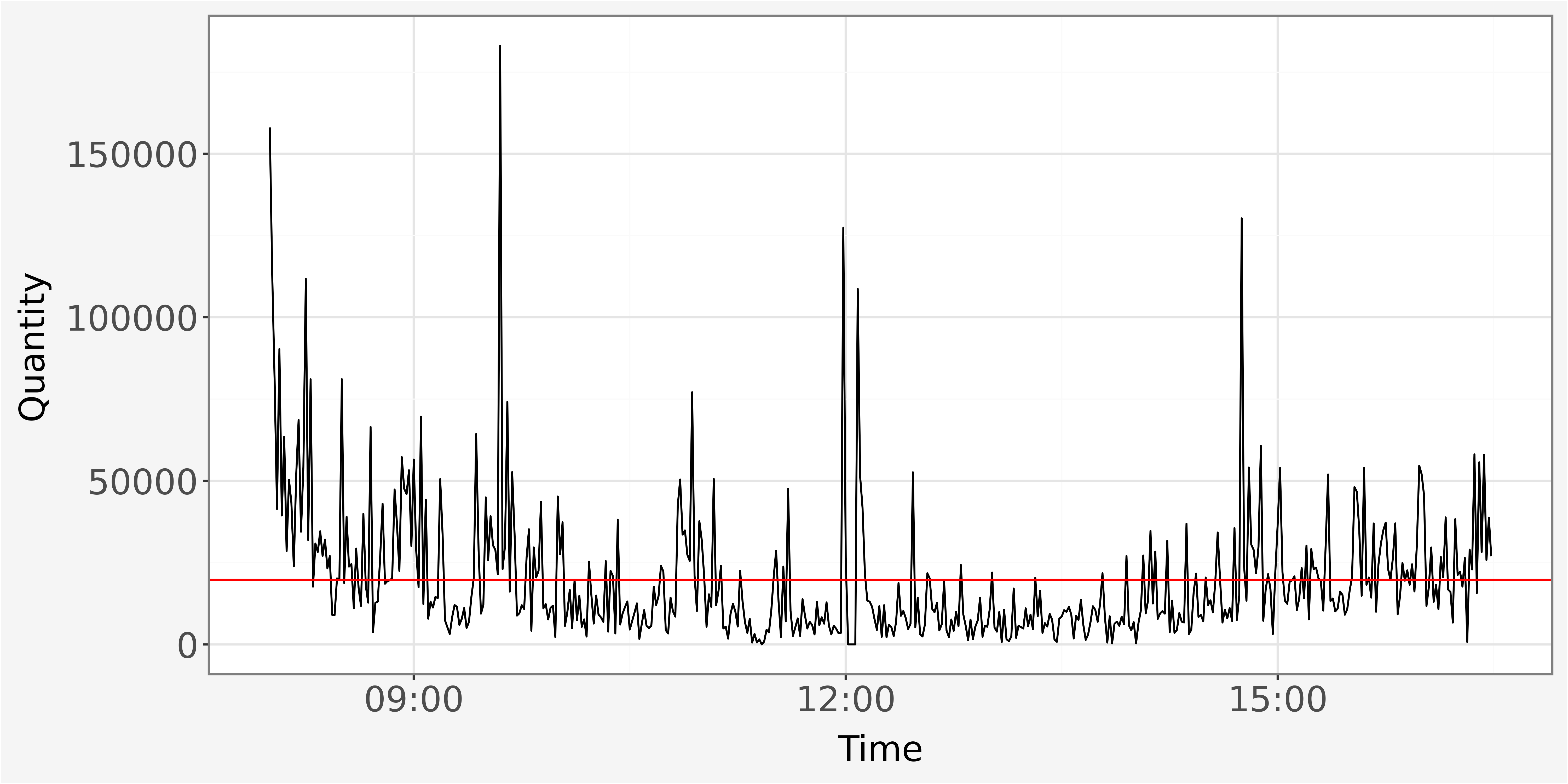
Plotting the execution sizes throughout the trading shows the typical diurnal U-shaped pattern, with increasing trading activity towards market opening and closing hours. The red line indicates the mean traded quantity per day.
Extreme movements in trading activity in the first hour of trading day can be caused by news transmitted over night. Trading activity slows down towards lunch time as overnight information is processed and diffused into price levels, but picks up again in the afternoon as traders re-balance their positions before market closure.
3.4.1 Missing Data
Handling missing data requires a a-priori definition of what missing data is. An entire row can be defined as being subject to missing data if only a single attribute is missing (not available). Such row might then be entirely excluded from the analysis or could still be used if it contains all relevant variables.
Dealing with missing data heavily depends on the context of the data and the type of the analysis. The final decision on how to deal with incomplete data should be made after computing the fraction of incomplete data within the dataset. Missing values can be interpolated, set to equal zero or discarded entirely.
We can either investigate the data for completeness by looking at the single rows in continuous time separately or investigate the completeness of the equi-distant discretized data. We focus on analyzing the discretized data for completeness. In our time series data, we could consider missing values as minute-timestamps which do not have any trading data available. This investigation can only be conducted after discretization of data and is not suitable for data in a continuous setting (unless you are interested in investigating single trade level missing data).
We start by defining the number of trading minutes for a single trading day we would expect given a complete dataset. Trading session starts at 8.00 am and closes at 4.30 pm, what makes a total of 510 intraday minutes. We then compare the number of trading minutes with the length of our discretized trade dataframe.
# Number of full trading minutes
trading_minutes = (16.5 - 8.0) * 60

# Number of full trading minutes versus number of rows in trades dataframe
print(f"""Number of trading minutes per day: {int(trading_minutes)} \nLength of trades dataframe: {len(trades_discretized)}""")
Number of trading minutes per day: 510
Length of trades dataframe: 510Comparing the length of the dataframe with the calculated number of trading minutes makes the data look complete. However, len() only counts the number of rows within the dataframe. It does not allow for inferences about whether the rows are in fact completed. We therefore use .isna() (is not available) and check whether the price is available for each of our minutes (equivalent to all our rows within the dataframe).
We identify five timestamps with missing values within the discretized trades dataframe, which we discard from further analysis.
# Subset the complete dataframe
trades_discretized_complete = trades_discretized[~trades_discretized["price_mean"].isna()]
print(f"Number of trades aggregated to low frequency: {len(trades_discretized_complete)}")
Number of trades aggregated to low frequency: 505Alternatively, we can utilize more advanced tools to handle missing values within our dataframe. We can drop the entire row which contains a a single missing observation within one colums. Such a rule is easily implemented, however might cause a significant loss of information in the following analysis. More advanced strategies contain the removal of reconrs which contain more (or less) than a predetermined threshold of (missing) values.
3.4.2 Duplicates
Identification of duplicate values is also highly dependent on the dataset and requires identification of a primary key which distinguishes between the different row entries. Since our data has been aggregated as a time series on a one-minute basis, we determine the timestamp as a unique identifier for the separate rows.
9165# Investigate how often each trade id occurs in dataframe
trades_grouped = trades.groupby("trade_id")["trade_timestamp"]\
.count()\
.reset_index()\
.sort_values("trade_timestamp")We see that some of the trade_id’s occur multiple times within our dataframe. We therefore pick one trade_id and analyse it in more detail.
This trade seems to be executed against numerous limit orders, as we observe multiple entries for the trade with a single trade_id. We use count to infer about the number of limit orders executed against the trade, mean indicates the average execution size per limit order, while sum indicates the sum of all shares traded within the timestamp.
# Investigate trade id occuring 71 times
one_trade = trades[trades["trade_id"] == 1582277957166155296]\
                .sort_values(["trade_timestamp",
                              "price",
                              "aggressor_side"])\
                .groupby(["trade_timestamp",
                          "price"])\
                .agg({"execution_size":["sum", "count", "mean"]})\
                .sort_values("trade_timestamp")\
                .reset_index()
3.5 Outliers
An outlier is an individual point of data that is distant from other points in the dataset. It is an anomaly in the dataset that may be caused by a range of errors in capturing, processing or manipulating data. The outlier is not necessarily due to erroneous measurements, but might be classified as contextual outlier which does not seem to have been produced by the underlying data generating process. Outliers can easily skew the data and cause bias in the development of the model.
| Point Outlier | In data analysis, a point outlier is an observation or data point that significantly differs from other observations in a dataset. Point outliers can occur due to measurement errors, data entry mistakes, or genuine deviations in the data. |
| Contextual Outlier | A contextual outlier is also known as conditional outlier and refers to an observation or data point that is unusual within a specific context of observation. This means that it is unusual within a certain (sub)sample of the dataset but may not be considered an outlier when looking at the entire dataset. |
| Collective Outlier | A collective outlier, also known as a group outlier or a contextual collective outlier, is a pattern or group of observations in a dataset that is significantly different from the rest of the data. |
To identify outliers we can use information about the inter-quantile range. The interquantile range is defined as distance between the third and the first quantile for a certain variable. By convention, observations which lie 1.5 times above (below) the third (first) quantile are removed.
cols = ['execution_size']

# Determine Quantiles
Q1 = trades[cols].quantile(0.25)
Q3 = trades[cols].quantile(0.75)

# Compute interquantile range
IQR = Q3 - Q1

# Remove observations outside of interquantile range
trades_filtered = trades[~((trades[cols] < (Q1 - 1.5 * IQR)) | (trades[cols] > (Q3 + 1.5 * IQR))).any(axis=1)].reset_index(drop=True)
Alternatively, we can winsorize the data. Winsorization describes the process of replacing extreme values of the data with a lower and upper bound limit. Such limit values are empirically derived from the data itself. A 90% winsorization indicates that bottom 5% and top 5% of the observable data has been set to 5th and 95th percentile of the empirically observed data. One advantage of using this method is that it does not discard any observations and therefore keeps a maximum of information within the data.
from scipy.stats import mstats

trades['execution_size_winsor'] = mstats.winsorize(trades['execution_size'], limits=[0.05, 0.05])
Finally, we can use mean or median imputation of the data. Mean (median) imputation replaces missing values with the mean (median) of the available data for the feature.
Imputation techniques are relatively simple to implement, however, they might not be appropriate for features with skewed distributions or outliers, as the mean can be influenced by extreme values. Both mean and median imputation are basic techniques and can introduce bias into the dataset, especially if the missing values are not missing at random. Data which is not missing at random requires an advanced invetigation of the dataset to find underlying reasons as to why the missing values occur.
3.6 Exercise
Discretization| (0) | Read the data from the corresponding .csv files. |
| (1) | Discretize the data from nanoseconds (\(10^{-9}\) of a second) to miliseconds (\(10^{-3}\) of a second), computing the sum and average traded quantity and traded volume, as well as the average price and number of trades executed per one-minute interval. |
| (2) | Discretize the data from nanoseconds (\(10^{-9}\) of a second) to seconds (\(10^{0}\) of a second). |
| (3) | Discretize the data from nanoseconds (\(10^{-9}\) of a second) to minutes. |
| (4) | On the discretized dataframe, compute one-minute logarithmic returns \(r_{t} = log(P_t) - log(P_{t-1})\) and one-minute logarithmic squared returns \(r_{t}^2 = [log(P_t) - log(P_{t-1})]^2\) for all intraday trading minutes with \(t \in [1,510]\). |
| (5) | On the undiscretized dataframe, compute the average duration between the execution of two consecutive trades. |
| (6) | On the undiscretized dataframe, add a new column to the dataframe named execution_size_sc. Compute the value of the newly added column as ratio between the traded quantity of a trade \(i\) and mean quantity per trade for the entire day \(execution\_size\_sc = \frac{traded_quantity_i}{\frac{1}{N} \sum^N_{i=1} traded\_quantity_i}\). \(N\) denotes the number of trades within the dataset. |
| (7) | For trades executed against multiple limit orders, what is the average duration it takes to fully execute the trade? Can you provide descriptives about the variable? |
Due to performance reasons, perform the following analysis on the one-minute discretized data.
| (8) | Plot the price series throughout the trading day. |
| (9) | Plot the return series throughout the trading day. |
| (10) | Plot an histogram of the returns series. What do you observe? |
| (11) | Plot the intraday volatility as the sum of squared returns \(\sigma_{r,t} = \sqrt{\sum_{i=1}^{n}r_i^2}\) with different values for the lookback parameter \(n=[5, 10, 15, 30, 60]\) (i.e., different frequencies 5-minutes, 10-minutes, 15-minutes, 30-minutes, 60-minutes). |
Now, go back to the indiscretized data on nanosecond level.
| (12) | Modify the dataframe in a way that it only contains one single row per trade_id instead of multiple rows with identical trade_id’s. Aggregate all relevant metrics on a trade level. Think of suitable and economically interpretable ways to aggregate the relevant metrics per trade. Additionally, count the number each trade_id occurs within the dataframe. What is the economic rationale behind a trade_id occurring multiple times in the dataframe? |
| (13) | Go back to section Visualization. Investigate the data more closely for potential anomalies. Do you find any outliers - if so where? Where do they come from? What statistical rule can you implement to identify them within the dataset? |
| (14) | Trade side classification algorithm: Create a new variable that indicates the direction of a trade. Assign the values of \(1\) for a buy and \(-1\) for a sell. According to the “quote rule” (QR), a trade is classified as buy if \(P_{trade,t} > P_{mid,t}\) with \(P_{trade}\) indicating the trade price and \(P_{mid}\) the midpoint. Analogously, a trade is classified as sell if \(P_{trade,t} < P_{mid,t}\). Whenever \(P_{trade,t} = P_{mid,t}\), the trade is not classified (Lee and Ready, 1991). How do your computed directions compare to the already given directions in the dataset? |
| (15) | Compute a set of descriptive statistics of your choice based on the dataset to infer about intraday trading activity and patterns. |