Chapter 5 建模
5.1 划分选来集合测试集合
bins <-  scorecard::woebin(cdata_reduced_2,y = 'label')
dt_woe <- scorecard::woebin_ply(cdata_reduced_2,bins)
## Woe transformating on 322715 rows and 11 columns in 00:00:12dt_woe$label <- as.factor(dt_woe$label)
div_part_1 <- createDataPartition(y = dt_woe$label, p = 0.7, list = F)
# Training Sample
train_1 <- dt_woe[div_part_1,] # 70% here
pct(train_1$label)| Count | Percentage | |
|---|---|---|
| 0 | 199708 | 88.41 |
| 1 | 26193 | 11.59 |
# Test Sample
test_1 <- dt_woe[-div_part_1,] # rest of the 30% data goes here
pct(test_1$label)| Count | Percentage | |
|---|---|---|
| 0 | 85589 | 88.41 |
| 1 | 11225 | 11.59 |
5.2 训练模型以及模型选择
5.2.1 逻辑回归以及逐步回归
m1 <- glm(label~.,data=train_1,family=binomial())
m1 <- step(m1)
## Start: AIC=141064.5
## label ~ 地址种类_woe + app1_woe + 下单与付款时间间隔_woe +
## cod运费_woe + 修改后金额_woe + 原始来单金额_woe +
## 金额差异_woe + 付款到派送_woe + 发货方式_woe +
## 用户性别_woe + 州_woe
##
##
## Step: AIC=141064.5
## label ~ 地址种类_woe + app1_woe + 下单与付款时间间隔_woe +
## cod运费_woe + 修改后金额_woe + 原始来单金额_woe +
## 付款到派送_woe + 发货方式_woe + 用户性别_woe +
## 州_woe
##
## Df Deviance AIC
## - 修改后金额_woe 1 141042 141062
## <none> 141042 141064
## - 原始来单金额_woe 1 141053 141073
## - cod运费_woe 1 141170 141190
## - 下单与付款时间间隔_woe 1 141309 141329
## - 州_woe 1 141389 141409
## - 发货方式_woe 1 141516 141536
## - 用户性别_woe 1 142610 142630
## - 付款到派送_woe 1 145987 146007
## - app1_woe 1 146280 146300
## - 地址种类_woe 1 146451 146471
##
## Step: AIC=141062.5
## label ~ 地址种类_woe + app1_woe + 下单与付款时间间隔_woe +
## cod运费_woe + 原始来单金额_woe + 付款到派送_woe +
## 发货方式_woe + 用户性别_woe + 州_woe
##
## Df Deviance AIC
## <none> 141042 141062
## - 原始来单金额_woe 1 141123 141141
## - cod运费_woe 1 141172 141190
## - 下单与付款时间间隔_woe 1 141309 141327
## - 州_woe 1 141389 141407
## - 发货方式_woe 1 141516 141534
## - 用户性别_woe 1 142610 142628
## - 付款到派送_woe 1 145988 146006
## - app1_woe 1 146280 146298
## - 地址种类_woe 1 146451 146469summary(m1)##
## Call:
## glm(formula = label ~ 地址种类_woe + app1_woe + 下单与付款时间间隔_woe +
## cod运费_woe + 原始来单金额_woe + 付款到派送_woe +
## 发货方式_woe + 用户性别_woe + 州_woe, family = binomial(),
## data = train_1)
##
## Deviance Residuals:
## Min 1Q Median 3Q Max
## -2.5995 -0.5347 -0.3976 -0.2337 3.8521
##
## Coefficients:
## Estimate Std. Error z value Pr(>|z|)
## (Intercept) -2.036266 0.007616 -267.35 <2e-16 ***
## 地址种类_woe 1.011125 0.021069 47.99 <2e-16 ***
## app1_woe 1.017471 0.015451 65.85 <2e-16 ***
## 下单与付款时间间隔_woe 0.952940 0.058721 16.23 <2e-16 ***
## cod运费_woe 0.529066 0.046369 11.41 <2e-16 ***
## 原始来单金额_woe 0.398816 0.044658 8.93 <2e-16 ***
## 付款到派送_woe 1.410965 0.021934 64.33 <2e-16 ***
## 发货方式_woe 0.807609 0.037204 21.71 <2e-16 ***
## 用户性别_woe 0.795311 0.019860 40.05 <2e-16 ***
## 州_woe 0.559377 0.030152 18.55 <2e-16 ***
## ---
## Signif. codes: 0 '***' 0.001 '**' 0.01 '*' 0.05 '.' 0.1 ' ' 1
##
## (Dispersion parameter for binomial family taken to be 1)
##
## Null deviance: 162095 on 225900 degrees of freedom
## Residual deviance: 141042 on 225891 degrees of freedom
## AIC: 141062
##
## Number of Fisher Scoring iterations: 7significant.variables <- summary(m1)$coeff[-1,4] < 0.01
names(significant.variables)[significant.variables == TRUE]## [1] "地址种类_woe" "app1_woe" "下单与付款时间间隔_woe"
## [4] "cod运费_woe" "原始来单金额_woe" "付款到派送_woe"
## [7] "发货方式_woe" "用户性别_woe" "州_woe"dt_pred = predict(m1, type='response', test_1)
perf_eva(test_1$label, dt_pred, type = c("ks","lift","roc","pr"))## Warning: Removed 1 rows containing missing values (geom_path).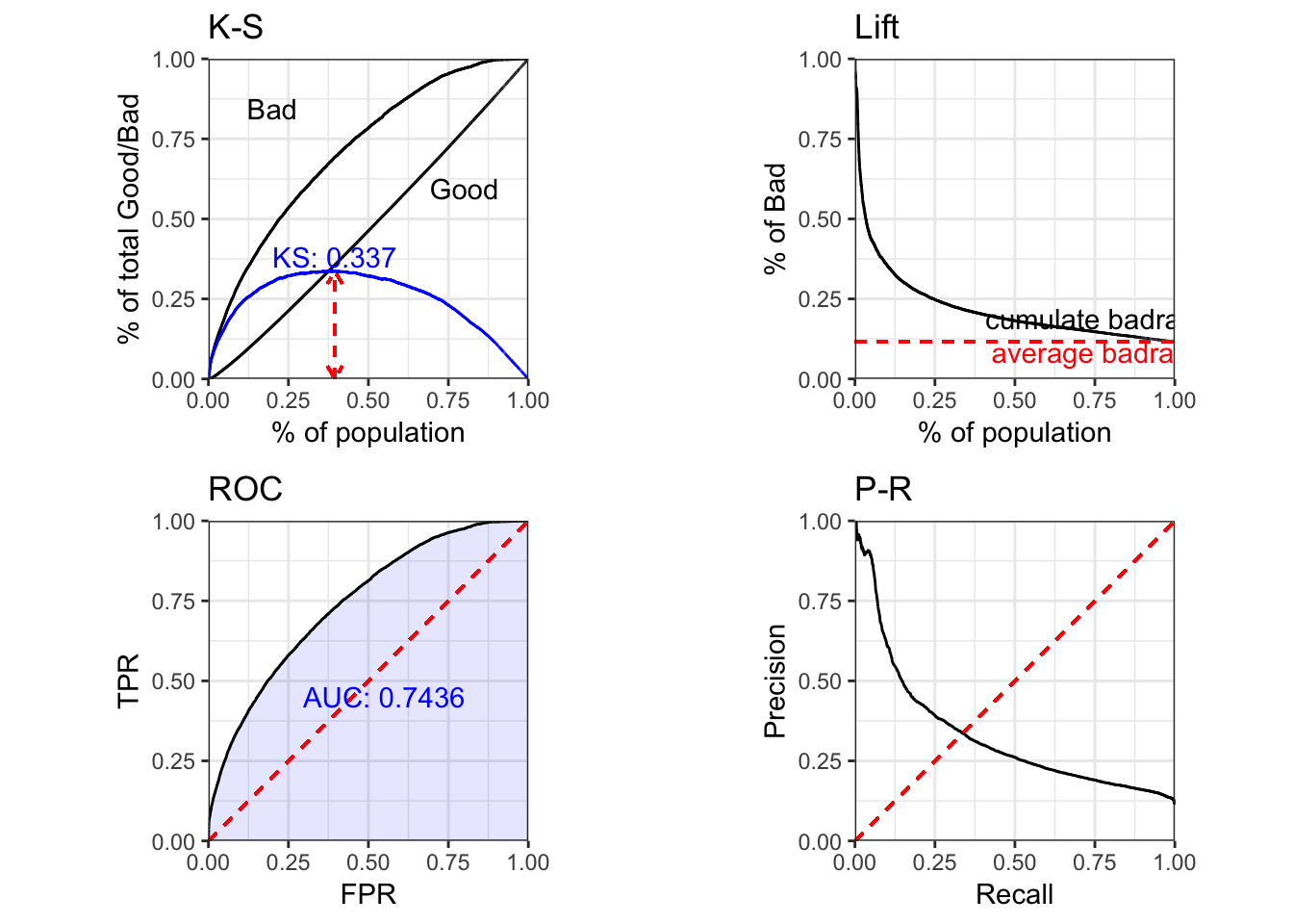
## $KS
## [1] 0.337
##
## $AUC
## [1] 0.7436
##
## $Gini
## [1] 0.4872
##
## $pic
## TableGrob (2 x 2) "arrange": 4 grobs
##       z     cells    name           grob
## pks   1 (1-1,1-1) arrange gtable[layout]
## plift 2 (1-1,2-2) arrange gtable[layout]
## proc  3 (2-2,1-1) arrange gtable[layout]
## ppr   4 (2-2,2-2) arrange gtable[layout]
5.2.2 随即森林
m3 <- randomForest(label ~ ., data = train_1)
par(family='STKaiti')
varImpPlot(m3, main="Random Forest: Variable Importance")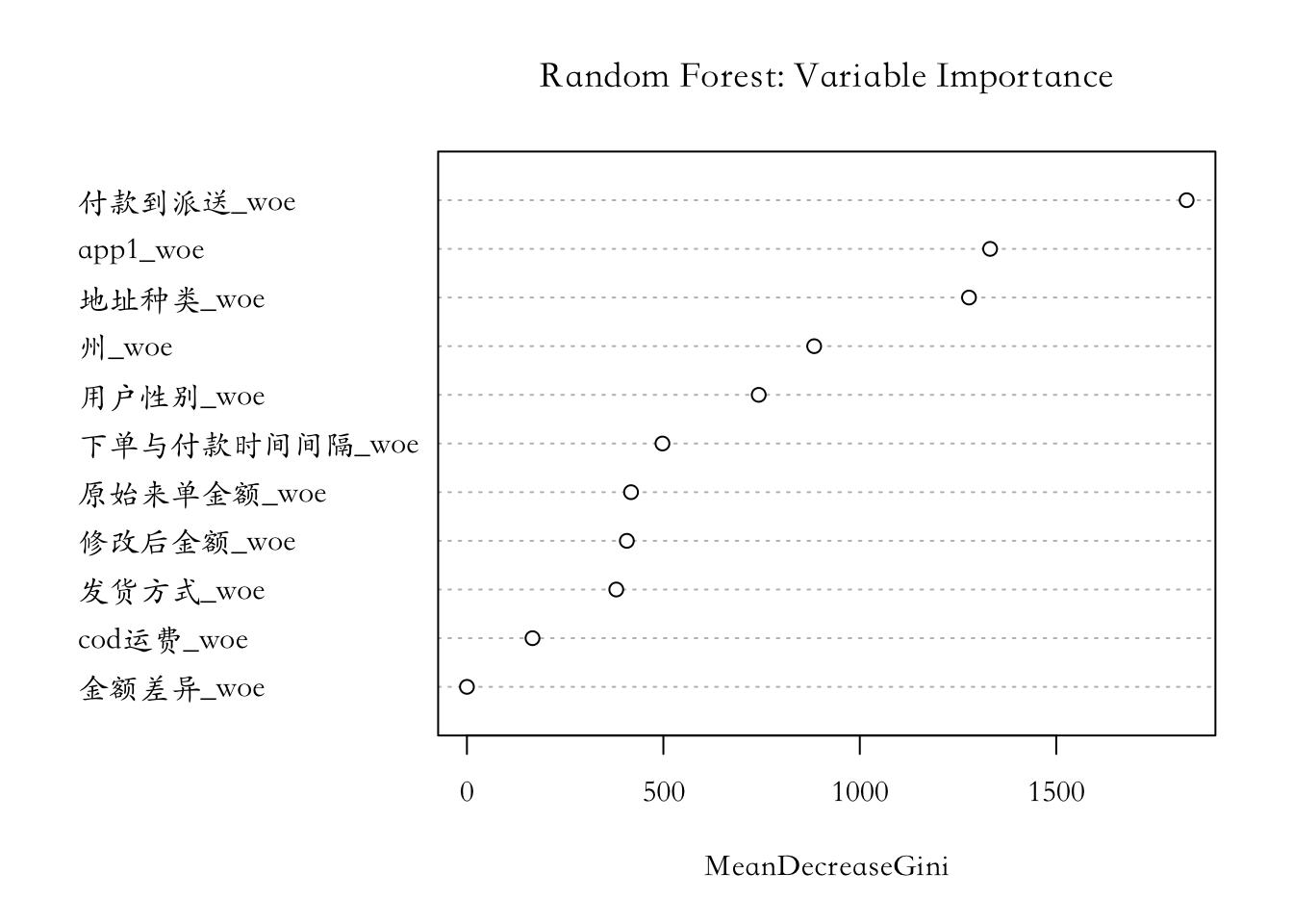
dt_pred = predict(m3, type='prob', test_1)[,1]
perf_eva(test_1$label, dt_pred, type = c("ks","lift","roc","pr"))
## Warning: Removed 1 rows containing missing values (geom_path).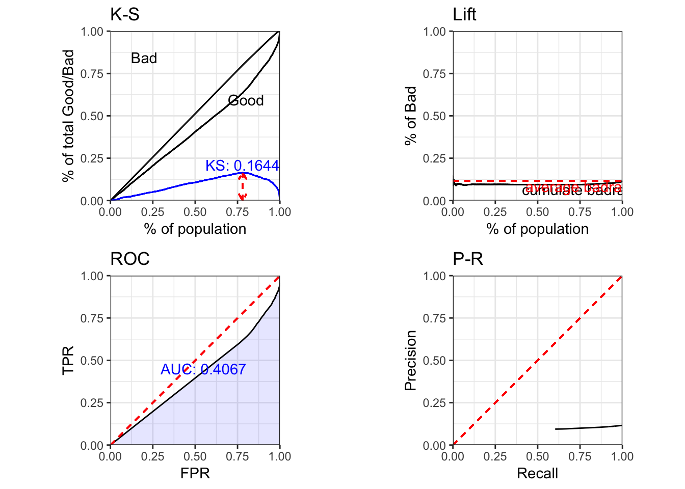
## $KS
## [1] 0.1644
##
## $AUC
## [1] 0.4067
##
## $Gini
## [1] -0.1866
##
## $pic
## TableGrob (2 x 2) "arrange": 4 grobs
##       z     cells    name           grob
## pks   1 (1-1,1-1) arrange gtable[layout]
## plift 2 (1-1,2-2) arrange gtable[layout]
## proc  3 (2-2,1-1) arrange gtable[layout]
## ppr   4 (2-2,2-2) arrange gtable[layout]
不平衡的数据会造成非常低AUC,需要尝试解决样本不平衡的问题
5.2.3 欠抽样
load('/Users/milin/COD\ 建模/model_rf_under.RData')
load('/Users/milin/COD\ 建模/dt_woe.RData')
require(scorecard)
dt_pred = predict(model_rf_under, type = 'prob', dt_woe)


perf_eva(dt_woe$label, dt_pred$`1`)
## $KS
## [1] 0.3986
##
## $AUC
## [1] 0.7641
##
## $Gini
## [1] 0.5281
##
## $pic
## TableGrob (1 x 2) "arrange": 2 grobs
##      z     cells    name           grob
## pks  1 (1-1,1-1) arrange gtable[layout]
## proc 2 (1-1,2-2) arrange gtable[layout]
5.2.3.1 重抽样
load('/Users/milin/COD\ 建模/model_rf_under1.RData')
dt_pred = predict(model_rf_under, type = 'prob', dt_woe)


perf_eva(dt_woe$label, dt_pred$`1`)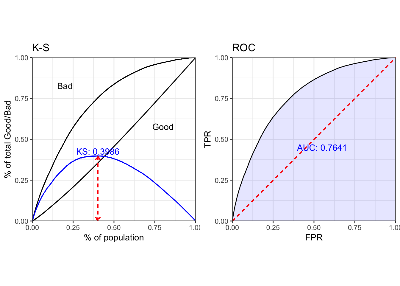
## $KS
## [1] 0.3986
##
## $AUC
## [1] 0.7641
##
## $Gini
## [1] 0.5281
##
## $pic
## TableGrob (1 x 2) "arrange": 2 grobs
##      z     cells    name           grob
## pks  1 (1-1,1-1) arrange gtable[layout]
## proc 2 (1-1,2-2) arrange gtable[layout]