Chapter 2 Refresh: Using R for data and spatial GIS
2.1 Introduction
This practical is intended as refresher for your spatial data handling skills in R/RStudio. It uses a series of worked examples to illustrate some fundamental and commonly applied operations on data and spatial datasets. It is based on Chapter 5 of Brunsdon and Comber (2018)1 and uses a series of worked examples to illustrate some fundamental and commonly applied spatial operations on spatial datasets. Many of these form the basis of most GIS software.
Specifically, in GIS and spatial analysis, we are often interested in finding out how the information contained in one spatial dataset relates to that contained in another. The datasets may be ones you have read into R from shapefiles or ones that you have created in the course of your analysis. Essentially, the operations illustrate different methods for extracting information from one spatial dataset based on the spatial extent of another. Many of these are what are frequently referred to as overlay operations in GIS software such as ArcGIS or QGIS, but here are extended to include a number of other types of data manipulation. The sections below describe how to create a point layer from a data table with location attributes and the following operations:
- Intersections and clipping one dataset to the extent of another
- Creating buffers around features
- Merging the features in a spatial dataset
- Point-in-Polygon and Area calculations
- Creating distance attributes
- Combining spatial data and attributes
2.1.1 Data
To do this, we will need some data and you can download and then load some data using the code below. This downloads data for Chapter 7 of Comber and Brunsdon (2021) from a repository
https://archive.researchdata.leeds.ac.uk/741/1/ch7.Rdata
download.file("https://archive.researchdata.leeds.ac.uk/741/1/ch7.Rdata",
              "./ch7.RData", mode = "wb")
You should see file called ch2.RData appear in your working directory and then you can load the data:
load("ch7.RData")Note that you can check where your working directory is by entering getwd() and you can change (reset) it by going to Session > Set Working Directory….
If you check what is is loaded you should see 2 R objects have been loaded into the session via the ch2.RData file.
ls()## [1] "lsoa" "oa" "properties"Three data files are loaded:
oaa multipolygonsfobject of Liverpool census Output Areas (OAs) (\(n = 1584\))lsoaa multipolygonsfobject of Liverpool census Lower Super Output Areas (LSOAs) (\(n = 298\))propertiesa pointsfobject scraped from Nestoria (https://www.nestoria.co.uk) (\(n = 4230\))
You can examine these in the usual way:
# look at the structure
str(oa)
str(lsoa)
# examine the first 6 rows
head(properties)
The census data attributes in oa and lsoa describe economic well-being (unemployment (the unmplyd attribute)), life-stage indicators (percentage of under 16 years (u16), 16-24 years (u25), 25-44 years (u45), 45-64 years (u65) and over 65 years (o65) and an environmental variable of the percentage of the census area containing greenspaces (gs_area). The unemployment and age data were from the 2011 UK population census (https://www.nomisweb.co.uk) and the greenspace proportions were extracted from the Ordnance Survey Open Greenspace layer (https://www.ordnancesurvey.co.uk/opendatadownload/products.html). The spatial frameworks were from the EDINA data library (https://borders.ukdataservice.ac.uk). The layer are projected to the OSGB projection (EPSG 27700) and has a geo-demographic class label (OAC) from the OAC (see https://data.cdrc.ac.uk/dataset/output-area-classification-2011).
We will work mainly with the oa and properties layers in this practical.
The properties data was downloaded on 30th May 2019 using an API (https://www.programmableweb.com/api/nestoria). It contains latitude (Lat) and longitude (Lon) in decimal degrees,allowing an sf point layer to be created from it, price in 1000s of pounds (£), the number of bedrooms and 38 binary variables indicating the presence of different keywords in the property listing such as Conservatory, Garage, Wood Floor etc.
The code below creates a flat data table from the properties point layer and then removes it. The idea in not having a spatial sf object propertiesbut a data table (like a spreadsheet) is similar to many real world situations - there is just a data table that you download, create, scrape or be sent (for example in your dissertation work).
# create a data frame version
props = data.frame(properties)
# check the names of the attributes
names(props)
## [1] "Kitchen" "Garden" "Modern"
## [4] "Gas.Central.Heating" "No.Chain" "Parking"
## [7] "Shared.Garden" "Double.Bedroom" "Balcony"
## [10] "New.Build" "Lift" "Gym"
## [13] "Porter" "Price" "Beds"
## [16] "Terraced" "Detached" "Semi.Detached"
## [19] "Conservatory" "Cul.de.Sac" "Bungalow"
## [22] "Garage" "Reception" "En.suite"
## [25] "Conversion" "Dishwasher" "Refurbished"
## [28] "Patio" "Cottage" "Listed"
## [31] "Fireplace" "Victorian" "Penthouse"
## [34] "Purpose.Built" "Wood.Floor" "Loft"
## [37] "Detached.Garage" "Auction" "Needs.Modernisation"
## [40] "Double.Garage" "geometry" "Lon"
## [43] "Lat"# remove the geometry attribute
props = props[, -41]
# remove the properties and lsao layers
rm(list = c("lsoa", "properties"))
# check what is present
ls()## [1] "oa" "props"Both of the remaining objects, oa and props have a data table format, with rows representing observations (people, places, dates, or in this cases census areas) and columns represent their attributes. Such long format data are the most commonly used and are similar to a standard spreadsheet, although the oa object is spatial and has geometries attached to each row, as do spatial data used in a GIS.
2.1.2 Packages
To handle these data types we will need some bespoke tools (functions) and these are found in packages. Recall that if you have not used packages on the computer your are working on before then they will need to be installed, using the install.packages function. The code below tests for the existence of the sf, tidyverse and tmap packages and installs them if they are not found:
# sf for spatial data
if (!is.element("sf", installed.packages()))
    install.packages("sf", dep = T)
# tidyverse for data handling and plotting
if (!is.element("tidyverse", installed.packages()))
    install.packages("tidyverse", dep = T)
# tmap for mapping
if (!is.element("tmap", installed.packages()))
    install.packages("tmap", dep = T)
# load the packages
library(sf)
library(tidyverse)
library(tmap)
2.2 Creating point data
The properties data props has locational attributes that can be used to convert it from a flat data table to point data.
This is the case in many situations and projects for which this - a flat data table - is the starting point: you are given a file with point observations of something (plus location) that you want to something spatial with.
The code converts the props flat table to the proprttties spatial object and undertakes this operation, using the WG84 projection for decimal degrees which has an EPSG code of 4236, noting that all projections have such a code2:
properties = st_as_sf(props, coords = c("Lon", "Lat"), crs = 4326)This can be plotted using a standard tmap approach:
tm_shape(properties) +
  tm_dots("Price", size = 0.1,alpha = 0.5,
          style = "kmeans",
          palette = "inferno") +
  tm_layout(bg.color = "grey95",
            legend.position = c("right", "top"),
legend.outside = T) 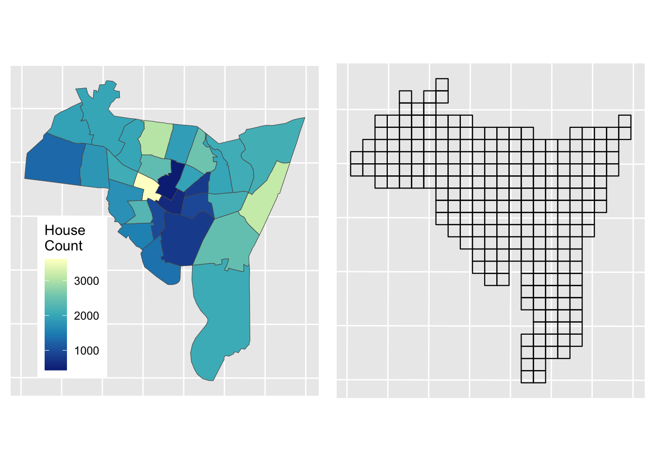
Figure 2.1: Proprties for sale in the Liverpool area.
Alternatively this can be done as an interactive map, by change the tmap_mode:
# set tmap mode for interactive plots
tmap_mode("view")
# create the plot
tm_shape(properties) +
  tm_dots("Price", alpha = 0.5,
          style = "kmeans",
          palette = "viridis") +
  tm_basemap("OpenStreetMap")
# reset tamp mode
tmap_mode("plot")
Figure 2.2: Interactive maps of Proprties for sale in the Liverpool area.
Task 1
Write some code that generates an interactive tmap of the number of bedrooms for the observations / records in the properties layer.
NB You are advised to attempt the tasks after the timetabled practical session. Worked answers are provided in the last section of the worksheet.
2.3 Intersections and Clip Operations
Now, consider the situation where the aim was to analyse the incidence of properties for sale in the Output Areas of Liverpool: we do not want to analyse all of the properties data but only those records that describe events in our study area - the area we are interested in.
This can be plotted using the usual commands as in the code below. You can see that the plot extent is defined by the spatial extent of area of interest (here oa) and that all of the properties within that extent are displayed.
# plot the areas
tm_shape(oa) +
  tm_borders(col = "black", lwd = 0.1) +
  # add the points
  tm_shape(properties) +
    tm_dots(col = "#FB6A4A") +
  # define some style / plotting oprions
  tm_layout(frame = F)
Figure 2.3: The OAs in Liverpool and the locations of properties for sale.
There are a number of ways of clipping spatial data in R. The simplest of these is to use the spatial extent of one as an index to subset another.
BUT to undertake any spatial operation with 2 spatial layers, they must be in the same projection. The tmap code above was able to handle this but spatial operations may fail.
Examine the properties layer and note its projection (particularly through the Geodetic CRS metadata at the top of the print out and the geometry attribute:
propertiesNow change the projection to OSGB3 and re-examine:
properties = st_transform(properties, 27700)
properties
The spatial extent of the liv layer can now be used to clip out the intersecting observations form the proprties layer:
prop_clip = properties[oa,]This simply clips out the data from properties that is within the spatial extent of oa. You can check this:
tm_shape(oa) +
  tm_fill() +
  tm_shape(prop_clip) +
  tm_dots()
However, such clip (or crop) operations simply subset data based on their spatial extents. There may be occasions when you wish to combine the attributes of difference datasets based on the spatial intersection. The st_intersection in sf allows us to do this as shown in the code below.
prop_int <- st_intersection(oa, properties)## Warning: attribute variables are assumed to be spatially constant throughout all
## geometriesThe st_intersection operation and the clip operation are based on spatial extents, do the same thing and the outputs are the same dimension but with subtle differences:
prop_clip
prop_int
If you examine the data created by the intersection, you will notice that each of the intersecting points has the full attribution from both input datasets (you may have to scroll up in your console to see this!):
head(data.frame(prop_clip))
head(data.frame(prop_int))
Task 2
Write some code that selects the polygon in oa with the LSOA code E00033902 (in the code attribute in oa) and then clips out the properties in that polygon. How many properties are there in E00033902?
NB You are advised to attempt the tasks after the timetabled practical session. Worked answers are provided in the last section of the worksheet.
2.4 Merging spatial features and Buffers
In many situations, we are interested in events or features that occur near to our area of interest as well as those within it. Environmental events such as tornadoes, for example, do not stop at state lines or other administrative boundaries. Similarly, if we were studying crimes locations or spatial access to facilities such as shops or health services, we would want to know about locations near to the study area border. Buffer operations provide a convenient way of doing this and buffers can be created in R using the st_buffer function in sf.
Continuing with the example above, we might be interested in extracting the properties within a certain distance of the Liverpool area, say 2km. Thus the objective is to create a 2km buffer around Liverpool and to use that to select from the properties dataset. The buffer function allow us to do that, and requires a distance for the buffer to be specified in terms of the units used in the projection.
The code below create a buffer, but does it for each OA - this is not we need in this case!
# apply a buffer to each object
buf_liv <- st_buffer(x = oa, dist = 2000)
# map
tm_shape(buf_liv) +
  tm_borders()
The code below uses st_union to merge all the OAs in liv to a single polygon and then uses that as the object to be buffered:
# union the oa layer to a single polygon
liv_merge <- st_sf(st_union(oa))
# buffer this
buf_liv <- st_buffer(liv_merge, 2000)
# and map
tm_shape(buf_liv) +
  tm_borders() +
  tm_shape(liv_merge) + tm_fill()
Figure 2.4: The outline of the Liverpool area (in grey) and a 2km buffer.
2.5 Point-in-polygon and Area calculations
2.5.1 Point-in-polygon
It is often useful to count the number of points falling within different zones in a polygon data set. This can be done using the the st_contains function in sf.
The code below returns a list of counts of the number properties that occur inside each OA to the variable prop.count and prints the first six of these to the console using the head function:
tmp = st_contains(oa, properties, sparse = F)
prop.count = rowSums(tmp)
head(prop.count)
## [1] 3 0 0 5 4 5length(prop.count)## [1] 1584Each of the observations in prop.count corresponds in order to the OAs in oa and could be attached to the data in the following way:
oa$prop.count = prop.countThis could be mapped using a full tmap approach as in the below, using best practice for counts (choropleths should only be used for rates!):
tm_shape(oa) +
  tm_dots(size = "prop.count", alpha = 0.5) +
  tm_shape(liv_merge) + tm_borders()
Figure 2.5: The the counts of properties for sale in the OAs in Liverpool.
2.5.2 Area calculations
Another useful operation is to be able calculate polygon areas. The st_area function in and sf does this. To check the projection, and therefore the map units, of an sf objects use the st_crs function:
st_crs(oa)This declares the projection to be in metres. To see the areas in square metres enter:
head(st_area(oa))These are not particularly useful and more realistic measures are to report areas in hectares or square kilometres:
# hectares
st_area(oa) / (100 * 100)
# square kilometres
st_area(oa) / (1000 * 1000)
Task 3
Your task is to create the code to produce maps of the densities of properties in each OA in Liverpool in properties per square kilometre. For the analysis you will need to use the properties point data and the oa dataset and undertake a point in polygon operation, apply an area function and undertake a conversion to square kilometres. The maps should be produced using the tm_shape and tm_fill functions in the tmap package^[Hint: in the tm_fill part of the mapping use style = "kmeans" to set the colour breaks).
NB You are advised to attempt the tasks after the timetabled practical session. Worked answers are provided in the last section of the worksheet.
2.6 Creating distance attributes
Distance is fundamental to spatial analysis. For example, we may wish to analyse the number of locations (e.g. health facilities, schools, etc) within a certain distance of the features we are considering. In the exercise below distance measures are used to evaluate differences in accessibility for different social groups, as recorded in census areas. Such approaches form the basis of supply and demand modelling and provide inputs into location-allocation models.
Distance could be approximated using a series of buffers created at specific distance intervals around our features (whether point or polygons). These could be used to determine the number of features or locations that are within different distance ranges, as specified by the buffers using the poly.counts function above. However distances can be measured directly and there a number of functions available in R to do this.
First, the most commonly used is the dist function. This calculates the Euclidean distance between points in \(n-\)dimensional feature space. The example below developed from the help for dist shows how it is used to calculate the distances between 5 records (rows) in a feature space of 20 hypothetical variables:
# create some random data
set.seed(123) # for reproducibility
x <- matrix(rnorm(100), nrow = 5)
colnames(x) <- paste0("Var", 1:20)
dist(x)
as.matrix(dist(x))
If your data is projected (i.e. in metres, feet etc) then dist can also be used to calculate the Euclidean distance between pairs of coordinates (i.e. 2 variables not 20!):
coords = st_coordinates(st_centroid(oa))
dmat = as.matrix(dist(coords, diag = F))
dim(dmat)
dmat[1:6, 1:6]
The distance functions return a to-from matrix of the distances between each pair of locations. These could describe distances between any objects and such approaches underpin supply and demand modelling and accessibility analyses.
When determining geographic distances, it is important that you consider the projection properties of your data: if the data are projected using degrees (i.e. in latitude and longitude) then this needs to be considered in any calculation of distance. The st_distance function in sf calculates the Cartesian minimum distance (straight line) distance between two spatial datasets of class sf projected in planar coordinates.
The code below calculates the distance between 2 features:
st_distance(oa[100,], properties[2,])## Units: [m]
## [,1]
## [1,] 3118.617And this can be extended to calculates multiple distances using a form of apply function. The code below uses st_distance to determine the distance from the 100^th observation in oa to each of the properties for sale:
g1 = st_geometry(oa[100,])
g2 = st_geometry(properties)
dlist = mapply(st_distance, g1, g2)
length(dlist)
## [1] 4230head(dlist)## [1] 4440.633 3118.617 10518.848 4435.707 2519.499 2519.499You could check this by mapping the properties data, shaded by their distance to this location:
tm_shape(cbind(properties, dlist)) +
  tm_dots("dlist", size = 0.1,alpha = 0.5,
          style = "kmeans",
          palette = "inferno") +
  tm_layout(bg.color = "grey95",
            legend.position = c("right", "top"),
            legend.outside = T) +
tm_shape(oa[100,]) + tm_borders("red", lwd = 4) 
Figure 2.6: A map of the proprties for sale inthe Liverpool area shaded by their distance to the 100th observation.
2.7 Combining spatial datasets and their attributes
The point-in-polygon calculation above generates counts of the points falling in each polygon. A common situation in spatial analysis is the need to combine (overlay) different polygon features that describe the spatial distribution of different variables, attributes or processes that are of interest. The problem is that the data may have different underlying area geographies. In fact, it is commonly the case that different agencies, institutions and government departments use different geographical areas and even where they do not, geographical areas frequently change over time.
In these situations, we can use the intersection function st_intersection in sf to identify the area of intersection between different spatial datasets.
In this exercise, a zone dataset will be created with the aim of calculating the number of of properties for sale in each zone. Now we could just use a point in polygon operation with the raw properties data in this case, but the aim here to illustrate the technique, when for example data are only available over a specific set of areas such as the Output Areas here.
First, you should create the zones, number them with an ID and plot these on a map with the OA data:
## define a 1km grid in polygons
sq = st_make_grid(oa, 1000, what = "polygons", square = T)
sq_grid = data.frame(ID = 1:length(sq))
st_geometry(sq_grid) = sq
# clip the extent of oa
sq_grid = sq_grid[oa,]
# plot
tm_shape(sq_grid) + tm_polygons(col = "grey") +
  tm_shape(oa) +tm_borders(col = "red")
Figure 2.7: A map of the the OAs (red) and the 1km grid.
The 2 layers, st_grid and oa have the same projections, and so they can be intersected using st_intersection:
int.res_sf <- st_intersection(sq_grid, oa[, c("code","prop.count")])## Warning: attribute variables are assumed to be spatially constant throughout all
## geometriesYou can examine the intersected data:
head(int.res_sf) You will see that the data.frame of the intersected object contains composites of the inputs. These links can be used to create attributes for the intersection output data.
First, note that the ID variable of int.res_sf relates to the ID variable of sq_grid and the variable prop.count is from the variable of the same name in oa. We wish to summarise this over the zones of sq_grid. Here the functionality of dplyr single table operations that were introduced in Chapter 4 can be useful. Knowing the the unique identifiers of each polygon in both of the intersected layers is critical for working out proportions.
# generate area and proportions
int.areas <- st_area(int.res_sf)
liv.areas <- st_area(oa)
# match tract area to the new layer
index <- match(int.res_sf$code, oa$code)
liv.areas <- liv.areas[index]
liv.prop <- as.vector(int.areas)/as.vector(liv.areas)
The liv.prop object can be used to create a variable in the data frame of the new layer
int.res_sf$props <- oa$prop.count[index] * liv.propAnd this can be summarised using the functionality in dplyr:
library(dplyr)
# summarise the counts of properties of the grid cells
int.res_sf %>% st_drop_geometry() %>%
  group_by(ID) %>%
  summarise(count = sum(props)) -> props
# link to the grid data
sq_grid %>% left_join(props) -> sq_grid
## Joining, by = "ID"The results can be plotted :
tm_shape(sq_grid) +
  tm_polygons("count", palette = "Greens",
              style = "kmeans", title = "Properties for sale") +
tm_layout(frame = F, legend.position = c(1,0.5)) 
Figure 2.8: The zones shaded by the number of propeties for sale after intersection with the Output Areas
Of course, all of this can be done using st_interpolate_aw which wraps up all of the above steps into a single function:
props2 = st_interpolate_aw(oa[, "prop.count"], sq_grid, extensive = T)
tm_shape(props2) +
  tm_polygons("prop.count", palette = "Greens",
              style = "kmeans", title = "No. of Properties for sale") +
  tm_layout(frame = F, legend.position = c(1,0.5))
2.8 Reading and writing data in and out of R/RStudio
There are 2 basic approaches:
- read and write data in and out of R/Rstudio in propriety formats such as shapefiles, CSV files etc.
- read and write data using
.Rdatafiles in R’s binary format and the load and save functions.
The code below provides does these as a reference for you:
Tabular data (CSV format)
write.csv(props, file = "props.csv", row.names = FALSE)
p2 = read.csv("props.csv", header=TRUE)
Tabular data (.RData format)
save(props, file = "props.RData")
load("props.RData") # notice that this needs no assignation e.g. to p2 or props
Spatial data (Proprietry format)
# as shapefile
st_write(properties, "point.shp", delete_layer = T)
p2 = st_read("point.shp")
# as GeoPackage
st_write(oa, "area.gpkg", delete_layer = T)
a2 = st_read("area.gpkg")
Spatial data (R format)
save(oa, file = "areas.RData")
load("areas.RData") # notice that this needs no assignation e.g. to p2 or props
2.9 Answer to Tasks
Task 1 Write some code that generates an interactive map of the number of bedrooms for the observations / records on properties.
# basic
tm_shape(properties) +
  tm_dots("Beds")
# with embellishment
tm_shape(properties) +
  tm_dots("Beds", size = 0.2, title = "Bedrooms",
          style = "kmeans", palette = "viridis") +
  tm_compass(bg.color = "white")+
  tm_scale_bar(bg.color = "white")
Task 2 Write some code that selects the polygon in oa with the LSOA code E00033902 (in the code attribute in oa) and then clips out the properties in that polygon. How many properties are there in E00033902?
## There are lots of ways of doing this but each of them uses a logical statement

# 1. using an index to create a subset and then clip
index = oa$code == "E00033902"
oa_select = oa[index,]
properties[oa_select,]

# 2. using the layer you have created already
sum(prop_int$code == "E00033902")
Task 3 Produce a map of the densities of properties for sale in each OA block in Liverpool in properties per square kilometre
# point in polygon
p.count <-  rowSums(st_contains(oa,properties,sparse = F))
# area calculation
oa.area <- st_area(oa) / (1000 * 1000)
# combine and assign to the liv data
oa$p.p.sqkm <- as.vector(p.count/oa.area)
# map
tm_shape(oa) +
  tm_fill("p.p.sqkm", style = "kmeans", title ="")
References
They can be found at https://epsg.io/ with this one being https://epsg.io/4326↩︎
EPSG 27700 - see https://epsg.io/27700↩︎