Chapter 2 Data and spatial data in R

2.1 Introduction

This practical is intended to refresh your spatial data handling skills in R/RStudio. It uses a series of worked examples to illustrate some fundamental and commonly applied operations on data and spatial datasets. It is based on Chapter 5 of Brunsdon and Comber (2018) and uses a series of worked examples to illustrate some fundamental and commonly applied spatial operations on spatial datasets. Many of these form the basis of most GIS software.

Specifically, in GIS and spatial analysis, we are often interested in finding out how the information contained in one spatial dataset relates to that contained in another. The datasets may be ones you have read into R from shapefiles or ones that you have created in the course of your analysis. Essentially, the operations illustrate different methods for extracting information from one spatial dataset based on the spatial extent of another. Many of these are what are frequently referred to as overlay operations in GIS software such as ArcGIS or QGIS, but here are extended to include a number of other types of data manipulation. The sections below describe how to create a point layer from a data table with location attributes and the following operations:

Intersections and clipping one dataset to the extent of another
Creating buffers around features
Merging the features in a spatial dataset
Point-in-Polygon and Area calculations
Creating distance attributes

An R script with all the code for this practical is provided.

2.1.1 Packages

To handle these data types we will need some bespoke tools (functions) and these are found in packages. Recall that if you have not used packages on the computer your are working on before then they will need to be installed, using the install.packages function. The code below tests for the existence of the sf, tidyverse and tmap packages and installs them if they are not found:

# tidyverse for data manipulation
if (!is.element("tidyverse", installed.packages()))
    install.packages("tidyverse", dep = T)# sf for spatial data
# sf for spatial data
if (!is.element("sf", installed.packages()))
    install.packages("sf", dep = T)
# tmap for mapping
if (!is.element("tmap", installed.packages()))
    install.packages("tmap", dep = T)

# load the packages
library(tidyverse)
library(sf)
library(tmap)

2.1.2 Data

To do this, we will need some data and you can download and then load some data using the code below. This downloads data for Chapter 7 of Comber and Brunsdon (2021) from a repository

https://archive.researchdata.leeds.ac.uk/741/1/ch7.Rdata

download.file("https://archive.researchdata.leeds.ac.uk/741/1/ch7.Rdata",
              "./wk1.RData", mode = "wb")

You should see file called wk1.RData appear in your working directory and then you can load the data:

load("wk1.RData")

Note that you can check where your working directory is by entering getwd() and you can change (reset) it by going to Session > Set Working Directory….

If you check what is is loaded you should see 3 objects have been loaded into the session via the wk1.RData file.

ls()

## [1] "lsoa"       "oa"         "properties"

Three data files are loaded:

oa a multipolygon sf object of Liverpool census Output Areas (OAs) (\(n = 1584\))
lsoa a multipolygon sf object of Liverpool census Lower Super Output Areas (LSOAs) (\(n = 298\))
properties a point sf object scraped from Nestoria (https://www.nestoria.co.uk) (\(n = 4230\))

You can examine these in the usual way:

# look at the structure
str(oa)
str(lsoa)
# examine the first 6 rows
head(properties)

You may get a warning about old-style crs object detected and you can run the code below to correct that:

properties <- st_transform(properties, 4326)

## old-style crs object detected; please recreate object with a recent sf::st_crs()

The census data attributes in oa and lsoa describe economic well-being (unemployment (the unmplyd attribute)), life-stage indicators (percentage of under 16 years (u16), 16-24 years (u25), 25-44 years (u45), 45-64 years (u65) and over 65 years (o65) and an environmental variable of the percentage of the census area containing greenspaces (gs_area). The unemployment and age data were from the 2011 UK population census (https://www.nomisweb.co.uk) and the greenspace proportions were extracted from the Ordnance Survey Open Greenspace layer (https://www.ordnancesurvey.co.uk/opendatadownload/products.html). The spatial frameworks were from the EDINA data library (https://borders.ukdataservice.ac.uk). The layer are projected to the OSGB projection (EPSG 27700) and has a geo-demographic class label (OAC) from the OAC (see https://data.cdrc.ac.uk/dataset/output-area-classification-2011).

We will work mainly with the oa and properties layers in this practical.

The properties data was downloaded on 30th May 2019 using an API (https://www.programmableweb.com/api/nestoria). It contains latitude (Lat) and longitude (Lon) in decimal degrees,allowing an sf point layer to be created from it, price in 1000s of pounds (£), the number of bedrooms and 38 binary variables indicating the presence of different keywords in the property listing such as Conservatory, Garage, Wood Floor etc.

The code below creates a flat data table in tibble format from the properties spatial point layer. The aim here is to have a simple data table with location attributes to work with

# create a tibble (like a data frame) of properties
props <- 
  properties |> st_drop_geometry() |> tibble()
# check
props

## # A tibble: 4,230 × 42
##    Kitchen Garden Modern `Gas Central Heating` `No Chain` Parking
##    <lgl>   <lgl>  <lgl>  <lgl>                 <lgl>      <lgl>  
##  1 FALSE   FALSE  FALSE  FALSE                 FALSE      FALSE  
##  2 FALSE   FALSE  FALSE  FALSE                 FALSE      FALSE  
##  3 FALSE   FALSE  FALSE  FALSE                 TRUE       FALSE  
##  4 TRUE    FALSE  FALSE  FALSE                 FALSE      TRUE   
##  5 TRUE    TRUE   FALSE  FALSE                 FALSE      TRUE   
##  6 FALSE   FALSE  FALSE  FALSE                 FALSE      FALSE  
##  7 FALSE   TRUE   FALSE  FALSE                 FALSE      FALSE  
##  8 TRUE    TRUE   FALSE  FALSE                 FALSE      TRUE   
##  9 TRUE    FALSE  FALSE  FALSE                 FALSE      TRUE   
## 10 TRUE    FALSE  TRUE   FALSE                 FALSE      FALSE  
## # ℹ 4,220 more rows
## # ℹ 36 more variables: `Shared Garden` <lgl>, `Double Bedroom` <lgl>,
## #   Balcony <lgl>, `New Build` <lgl>, Lift <lgl>, Gym <lgl>, Porter <lgl>,
## #   Price <dbl>, Beds <ord>, Terraced <lgl>, Detached <lgl>,
## #   `Semi-Detached` <lgl>, Conservatory <lgl>, `Cul-de-Sac` <lgl>,
## #   Bungalow <lgl>, Garage <lgl>, Reception <lgl>, `En suite` <lgl>,
## #   Conversion <lgl>, Dishwasher <lgl>, Refurbished <lgl>, Patio <lgl>, …

# remove the original layer and check
rm(properties)
ls()

## [1] "lsoa"  "oa"    "props"

Examining props shows that it has 4,230 observations and 42 fields or attributes. This is as standard flat data table format, with rows representing observations (people, places, dates, or in this cases census areas) and columns represent their attributes.

Note: Piping The syntax above uses piping syntax (|>) to pass the outputs of one function to the input of another. We will cover this syntax in more detail next week. But for now note that the two functions st_drop_geometry() and tibble() both have a data table of some kind as the first argument.

2.2 Using R as a GIS

2.2.1 Creating point data

The properties data props has locational attributes, Lat and Lon that can be used to convert it from a flat data table to point data using the st_as_sf() function:

# check the names
names(props)

# pass them in to the function as the `coords` parameter
properties = st_as_sf(props, coords = c("Lon", "Lat"), crs = 4326)

Note the use of crs = 4326: this specifies the projection of the coordinates in the Lat and Lon attributes. Here we know they are WGS84 the global standard for location, in which location is recorded in decimal degrees (see https://en.wikipedia.org/wiki/World_Geodetic_System), and the EPSG code for WGS84 is 4326 (https://epsg.io/4326))

This can be plotted using a standard tmap approach using the code below. This has a standard format of tm_shape(<spatial layer name>) + tm_plot_type(<attribute name>), which we will covered in detail in the self-directed part of this practical.

tm_shape(properties) + 
  tm_dots("Price", size = 0.1,alpha = 0.5, 
          style = "kmeans",
          palette = "inferno") + 
  tm_layout(bg.color = "grey95",
            legend.position = c("right", "top"),
            legend.outside = T)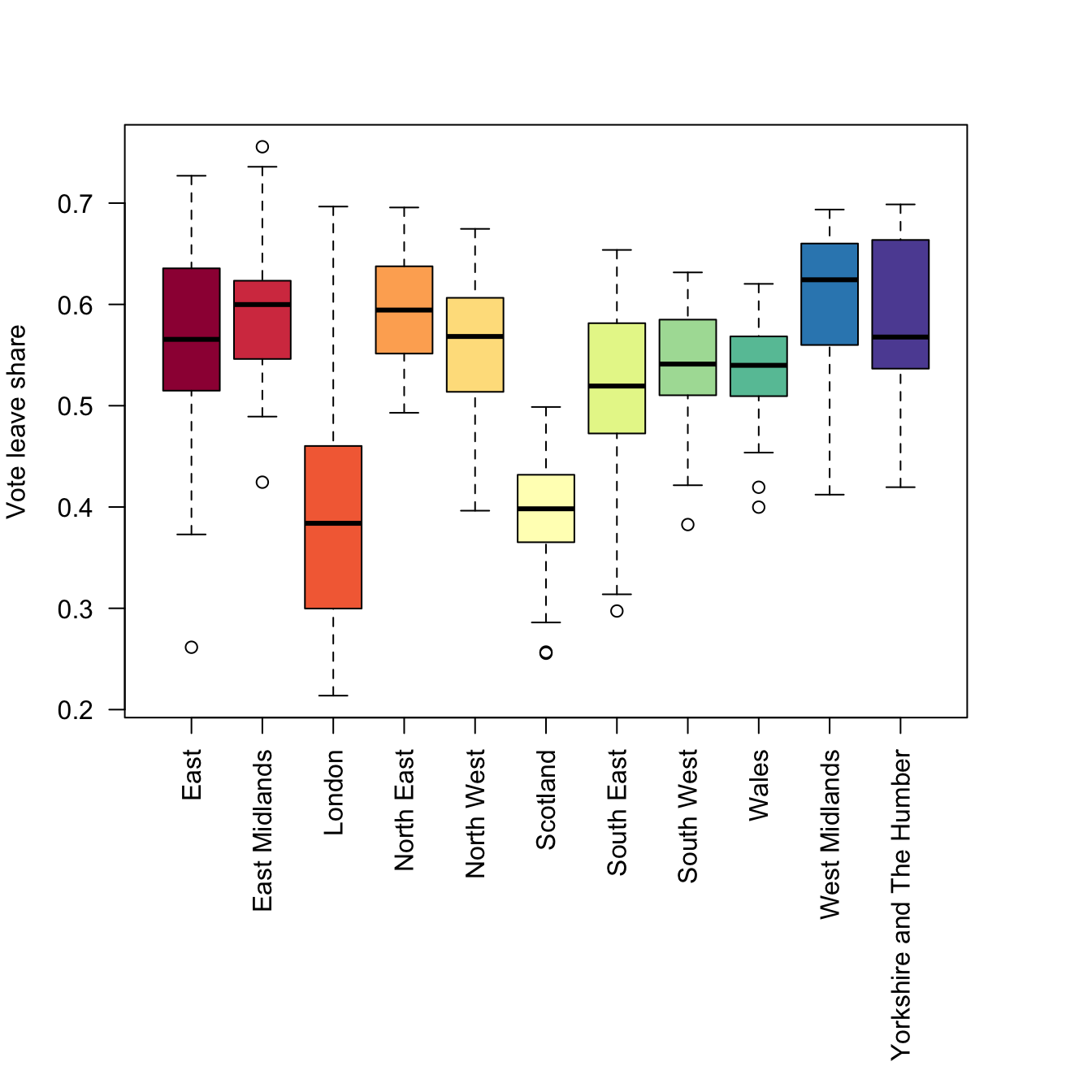

Figure 2.1: Proprties for sale in the Liverpool area.

Alternatively this can be done as an interactive map, by change the tmap_mode:

# set tmap mode for interactive plots
tmap_mode("view")
# create the plot
tm_shape(properties) + 
  tm_dots("Price", alpha = 0.5, 
          style = "kmeans",
          palette = "viridis") + 
  tm_basemap("OpenStreetMap")

# reset tamp mode
tmap_mode("plot")

Task 1

Write some code that generates an interactive tmap of the number of bedrooms for the observations / records in the properties layer.

NB You could attempt the tasks after the timetabled practical session. Worked answers are provided in the last section of the worksheet.

2.2.2 Spatial Operations

Now, consider the situation where the aim was to analyse the incidence of properties for sale in the Output Areas of Liverpool: we do not want to analyse all of the properties data but only those records that describe events in our study area - the area we are interested in.

This can be plotted using the usual commands as in the code below. You can see that the plot extent is defined by the spatial extent of area of interest (here oa) and that all of the properties within that extent are displayed.

# plot the areas
tm_shape(oa) +
  tm_borders(col = "black", lwd = 0.1) +
  # add the points 
  tm_shape(properties) +
    tm_dots(col = "#FB6A4A") +
  # define some style / plotting options
  tm_layout(frame = F)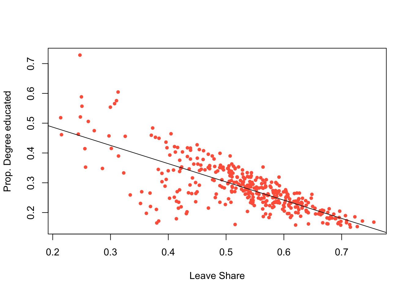

Figure 2.2: The OAs in Liverpool and the locations of properties for sale.

There are a number of ways of clipping spatial data in R. The simplest of these is to use the spatial extent of one as an index to subset another.

BUT to undertake any spatial operation with 2 spatial layers, they must be in the same projection. The tmap code above was able to handle the different projections of oa and proprties but spatial operations will fail. Examine the properties layer and note its projection, particularly through the Bounding box and Geodetic CRS or Projected CRS metadata at the top of the print out and the geometry attributes:

oa
properties

Now change the projection of properties to the Ordnance Survey OSGB projection (EPSG 27700 - see https://epsg.io/27700) and re-examine:

properties = st_transform(properties, 27700)
properties

The spatial extent of the oa layer can now be used to clip out the intersecting observations form the proprties layer:

prop_clip = properties[oa,]

This simply clips out the data from properties that is within the spatial extent of oa. You can check this:

tm_shape(oa) +
  tm_fill() +
  tm_shape(prop_clip) +
  tm_dots()

However, such clip (or crop) operations simply subset data based on their spatial extents. There may be occasions when you wish to combine the attributes of difference datasets based on the spatial intersection. The st_intersection in sf allows us to do this as shown in the code below.

prop_int <- st_intersection(oa, properties)

## Warning: attribute variables are assumed to be spatially constant throughout
## all geometries

The st_intersection operation and the clip operation are based on spatial extents, do the same thing and the outputs are the same dimension but with subtle differences:

prop_clip
prop_int

If you examine the data created by the intersection, you will notice that each of the intersecting points has the full attribution from both input datasets (you may have to scroll up in your console to see this!):

head(data.frame(prop_clip))
head(data.frame(prop_int))

Task 2

Write some code that selects the polygon in oa with the LSOA code E00033902 (in the code attribute in oa) and then clips out the properties in that polygon. How many properties are there in E00033902?

2.2.3 Merging spatial features and Buffers

In many situations, we are interested in events or features that occur near to our area of interest as well as those within it. Environmental events such as tornadoes, for example, do not stop at state lines or other administrative boundaries. Similarly, if we were studying crimes locations or spatial access to facilities such as shops or health services, we would want to know about locations near to the study area border. Buffer operations provide a convenient way of doing this and buffers can be created in R using the st_buffer function in sf.

Continuing with the example above, we might be interested in extracting the properties within a certain distance of the Liverpool area, say 2km. Thus the objective is to create a 2km buffer around Liverpool and to use that to select from the properties dataset. The buffer function allow us to do that, and requires a distance for the buffer to be specified in terms of the units used in the projection.

The code below create a buffer, but does it for each OA - this is not we need in this case!

# apply a buffer to each object
buf_liv <- st_buffer(x = oa, dist = 2000)
# map
tm_shape(buf_liv) + 
  tm_borders()

The code below uses st_union to merge all the OAs in oa to a single polygon and then uses that as the object to be buffered:

# union the oa layer to a single polygon
liv_merge <- st_sf(st_union(oa))
# buffer this
buf_liv <- st_buffer(liv_merge, 2000)
# and map
tm_shape(buf_liv) + 
  tm_borders() +
  tm_shape(liv_merge) + tm_fill()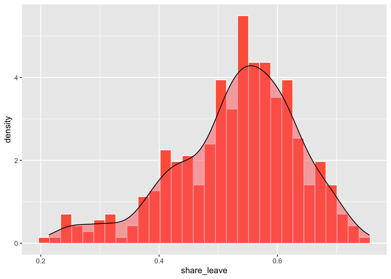

Figure 2.3: The outline of the Liverpool area (in grey) and a 2km buffer.

2.2.4 Point-in-polygon and Area calculations

2.2.4.1 Point-in-polygon

It is often useful to count the number of points falling within different zones in a polygon data set. This can be done using the the st_contains function in sf.

The code below returns a list of counts of the number properties that occur inside each OA to the variable prop.count and prints the first six of these to the console using the head function:

tmp = st_contains(oa, properties, sparse = F)
prop.count = rowSums(tmp)
head(prop.count)

## [1] 3 0 0 5 4 5

length(prop.count)

## [1] 1584

Each of the observations in prop.count corresponds in order to the OAs in oa and could be attached to the data in the following way:

oa$prop.count = prop.count

This could be mapped using a full tmap approach as in the below, using best practice for counts (choropleths should only be used for rates!):

tm_shape(oa) + 
  tm_dots(size = "prop.count", alpha = 0.5) +
  tm_shape(liv_merge) + tm_borders()

Figure 2.4: The the counts of properties for sale in the OAs in Liverpool.

2.2.4.2 Area calculations

Another useful operation is to be able calculate polygon areas. The st_area function in and sf does this. To check the projection, and therefore the map units, of an sf objects use the st_crs function:

st_crs(oa)

This declares the projection to be in metres. To see the areas in square metres enter:

head(st_area(oa))

These are not particularly useful and more realistic measures are to report areas in hectares or square kilometres:

# hectares
st_area(oa) / (100 * 100)
# square kilometres
st_area(oa) / (1000 * 1000)

Task 3

Your task is to create the code to produce maps of the densities of properties in each OA in Liverpool in properties per square kilometre. For the analysis you will need to use the properties point data and the oa dataset and undertake a point in polygon operation, apply an area function and undertake a conversion to square kilometres. The maps should be produced using the tm_shape and tm_fill functions in the tmap package (Hint: in the tm_fill part of the mapping use style = "kmeans" to set the colour breaks).

2.2.5 Creating distance attributes

Distance is fundamental to spatial analysis. For example, we may wish to analyse the number of locations (e.g. health facilities, schools, etc) within a certain distance of the features we are considering. In the exercise below distance measures are used to evaluate differences in accessibility for different social groups, as recorded in census areas. Such approaches form the basis of supply and demand modelling and provide inputs into location-allocation models.

Distance could be approximated using a series of buffers created at specific distance intervals around our features (whether point or polygons). These could be used to determine the number of features or locations that are within different distance ranges, as specified by the buffers using the poly.counts function above. However distances can be measured directly and there a number of functions available in R to do this.

First, the most commonly used is the dist function. This calculates the Euclidean distance between points in \(n-\)dimensional feature space. The example below developed from the help for dist shows how it is used to calculate the distances between 5 records (rows) in a feature space of 20 hypothetical variables:

# create some random data
set.seed(123) # for reproducibility
x <- matrix(rnorm(100), nrow = 5)
colnames(x) <- paste0("Var", 1:20)
dist(x)
as.matrix(dist(x))

If your data is projected (i.e. in metres, feet etc) then dist can also be used to calculate the Euclidean distance between pairs of coordinates (i.e. 2 variables not 20!):

coords = st_coordinates(st_centroid(oa)) 
dmat = as.matrix(dist(coords, diag = F))
dim(dmat)
dmat[1:6, 1:6]

The distance functions return a to-from matrix of the distances between each pair of locations. These could describe distances between any objects and such approaches underpin supply and demand modelling and accessibility analyses. When determining geographic distances, it is important that you consider the projection properties of your data: if the data are projected using degrees (i.e. in latitude and longitude) then this needs to be considered in any calculation of distance. The st_distance function in sf calculates the Cartesian minimum distance (straight line) distance between two spatial datasets of class sf projected in planar coordinates.

The code below calculates the distance between 2 features:

st_distance(oa[100,], properties[2,])

## Units: [m]
##          [,1]
## [1,] 3118.617

And this can be extended to calculates multiple distances using a form of apply function. The code below uses st_distance to determine the distance from the 100^th observation in oa to each of the properties for sale:

g1 = st_geometry(oa[100,])
g2 = st_geometry(properties) 
dlist = mapply(st_distance, g1, g2)
length(dlist)

## [1] 4230

head(dlist)

## [1]  4440.633  3118.617 10518.848  4435.707  2519.499  2519.499

You could check this by mapping the properties data, shaded by their distance to this location:

tm_shape(cbind(properties, dlist)) +
  tm_dots("dlist", size = 0.1,alpha = 0.5, 
          style = "kmeans",
          palette = "inferno") + 
  tm_layout(bg.color = "grey95",
            legend.position = c("right", "top"),
            legend.outside = T) + 
  tm_shape(oa[100,]) + tm_borders("red", lwd = 4)

Figure 2.5: A map of the proprties for sale inthe Liverpool area shaded by their distance to the 100th observation.

2.2.6 Reading and writing data in and out of R/RStudio

There are 2 basic approaches:

read and write data in and out of R/Rstudio in propriety formats such as shapefiles, CSV files etc.
read and write data using .Rdata files in R’s binary format and the load and save functions.

The code below provides does these as a reference for you:

Tabular data (CSV format)

write.csv(props, file = "props.csv", row.names = FALSE)
p2 = read.csv("props.csv", header=TRUE)

Tabular data (.RData format)

save(props, file = "props.RData")
load("props.RData") # notice that this needs no assignation e.g. to p2 or props

Spatial data (Proprietary format)

# as shapefile
st_write(properties, "point.shp", delete_layer = T)
p2 = st_read("point.shp")
# as GeoPackage
st_write(oa, "area.gpkg", delete_layer = T)
a2 = st_read("area.gpkg")

Spatial data (R format)

save(oa, file = "areas.RData")
load("areas.RData") # notice that this needs no assignation e.g. to p2 or props

2.3 Answer to Tasks

Task 1 Write some code that generates an interactive map of the number of bedrooms for the observations / records on properties.

# Task 1
# basic
tm_shape(properties) + 
  tm_dots("Beds") 
# with embellishment
tm_shape(properties) + 
  tm_dots("Beds", size = 0.2, title = "Bedrooms",
          style = "kmeans", palette = "viridis") +
  tm_compass(bg.color = "white")+
  tm_scale_bar(bg.color = "white")

Task 2 Write some code that selects the polygon in oa with the LSOA code E00033902 (in the code attribute in oa) and then clips out the properties in that polygon. How many properties are there in E00033902?

# Task 2
## There are lots of ways of doing this but each of them uses a logical statement

# 1. using an index to create a subset and then clip
index = oa$code == "E00033902"
oa_select = oa[index,]
properties[oa_select,]

# 2. using the layer you have created already 
sum(prop_int$code == "E00033902")

Task 3 Produce a map of the densities of properties for sale in each OA block in Liverpool in properties per square kilometre

# Task 3
# point in polygon
p.count <-  rowSums(st_contains(oa,properties,sparse = F))
# area calculation
oa.area <- st_area(oa) / (1000 * 1000)
# combine and assign to the oa data
oa$p.p.sqkm <- as.vector(p.count/oa.area)
# map
tm_shape(oa) +
  tm_fill("p.p.sqkm", style = "kmeans", title ="")

2.4 Optional: mapping with `tmap`

You will need to download the data_gb.geojson layer from the VLE.

We have been using tmap in the above exercises without really commenting on what is being done. This section covers mapping in tmap in a bit more detail.

The code below loads the Local Authority Districts (LADs) in Great Britain with attributes describing the Brexit vote and additional demographic data. You will need to have the data_gb.geojson in your working directory on your computer:

This is the same data and variables used in the analysis of the Brexit vote by Beecham, Williams, and Comber (2020). You can inspect in the usual way

summary(data_gb)
str(data_gb)

2.4.1 Mapping with `tmap`

The tmap package supports the thematic visualization of spatial data. It has a grammatical style that handles each element of the map separately in a series of layers (it is similar to ggplot in this respect - see below). In so doing it seeks to exercise control over each element in the map. This is different to the basic R plot functions. The basic syntax of tmap is:

tm_shape(data = <data>)+
  tm_<function>()

NB do not run the code above - its is simply showing the syntax of tmap. However, you have probably noticed that it uses a syntactical style similar to ggplot to join together layers of commands, using the + sign. The tm_shape function initialises the map and then layer types, the variables that get mapped etc, are specified using different flavours of tm_<function>. The main types are listed in the table below.

## 
## Attaching package: 'kableExtra'

## The following object is masked from 'package:dplyr':
## 
##     group_rows

Table 2.1: Commonly used `tmap` functions
Function	Description
tm_dots, tm_bubbles	for points either simple or sized according to a variable
tm_lines	for line features
tm_fill, tm_borders, tm_polygons	for polygons / areas, with and without attributes and polygon outlines
tm_text	for adding text to map features
tm_format, tm_facet, tm_layout	for adjusting cartographic appearance and map style, including legends
tm_view, tm_compass, tm_credits, tm_scale_bar	for including traditional cartography elements

Let’s start with a simple choropleth map. These show the distribution of a continuous variable in the spatial data (typically polygons / areas or points)

tm_shape(data_gb)+
  tm_polygons("share_leave")

Figure 2.6: A choropleth map of share_leave.

By default tmap picks a shading scheme, the class breaks and places a legend somewhere. All of these can be changed. The code below allocates the tmap plot to p1 (plot 1) and then prints it:

p1 = tm_shape(data_gb) + 
  tm_polygons("share_leave", palette = "GnBu", border.col = "salmon",
    breaks = seq(0,0.8, 0.1), title = "Leave Share")+
  tm_layout(legend.position = c("right", "top"), frame = F)
p1

And of course many other elements included either by running the code snippet defining p1 above with additional lines or by simply adding them as in the code below

p1 + 
  tm_scale_bar(position = c("left", "top")) + 
  tm_compass(position = c(0.15, 0.9))

It is also possible to add or overlay other data such as the region boundaries, which because this is another spatial data layer needs to be added with tm_shape followed by the usual function. Notice the use of the piping syntax to create regions:

# first make the region boundaries
regions <- data_gb %>% group_by(Region) %>% summarise()

# then add to the plot
p1 + tm_shape(regions) + tm_borders(col = "black", lwd = 1)

The tmap package can be used to plot multiple attributes in the same plot in this case the leave share and degree educated proportions:

tm_shape(data_gb)+
  tm_fill(c("share_leave", "degree_educated"), palette = "YlGnBu",
    breaks = seq(0,1, 0.1), title = c("Leave Share", "Degree"))+
  tm_layout(legend.position = c("left", "bottom"))

Figure 2.7: Choropleth maps of share_leave and degree_educated.

The code below applies further refinements to the code to generate the next map. Notice the use of title and legend.hist, and then subsequent parameters passed to tm_layout to control the legend:

tm_shape(data_gb)+
  tm_polygons("share_leave", title = "Leave Share", palette = "Reds",
    style = "kmeans", legend.hist = T)+
  tm_layout(title = "Leave Vote Share \nin the UK",
            frame = F, legend.outside = T, 
            legend.hist.width = 1,
            legend.format = list(digits = 1), 
            legend.outside.position = c("left", "top"),
            legend.text.size = 0.7,
            legend.title.size = 1) +
  tm_scale_bar(position = c("left", "top")) + 
  tm_compass(position = c("left", "top")) +
  tm_shape(regions) + tm_borders(col = "black", lwd = 1)

Figure 2.8: A refined choropleth map of the Leave Share.

This is quite a lot of code to unpick. The first call to tm_shape determines which layer is to be mapped, then a specific mapping function is applied to that layer (in this case tm_polygons) and a variable is passed to it. Other parameters are used to specify are the palette, whether a histogram is to be displayed and the type of breaks to be imposed (here a \(k\)-means was applied). The help for tm_polygons describes a number of different parameters that can be passed to tmap elements. Next, some adjustments were made to the defaults through the tm_layout function, which allows you to override the defaults that tmap automatically assigns (shading scheme, legend location etc). Finally the region layer was added.

There are literally 1000’s of options with tmap and many of them are controlled in the tm_layout function. You should inspect this:

?tm_layout

The code below creates and maps point data values in different ways. There are 2 basic options: change the size or change the shading of the points according to the attribute value. The code snippets below illustrate these approaches.

Create the point layer:

lads_pts = st_centroid(data_gb)

Then map by size using tm_bubbles as in the figure below:

tm_shape(regions) +
  tm_fill("olivedrab4") +
  tm_borders("grey", lwd = 1) + 
  # the points layer
  tm_shape(lads_pts) +
  tm_bubbles("share_leave", title.size = "Leave Vote", scale = 0.6, col = "gold") +
  tm_layout(legend.position = c("left", "top"))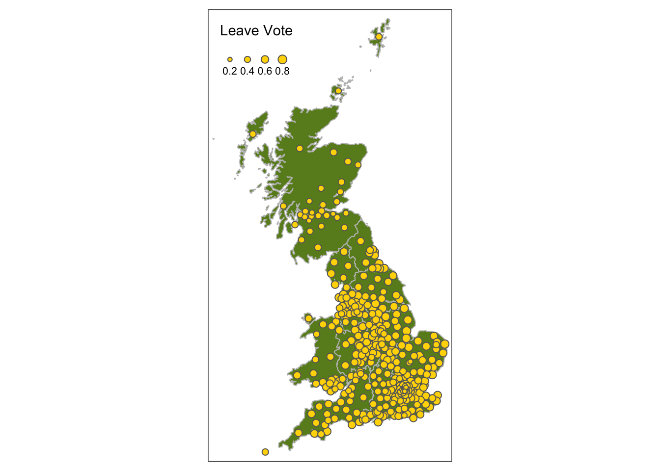

Figure 2.9: Point data values using size.

Second by shade using tm_dots as below:

# the 1st layer
tm_shape(regions) +
  tm_fill("grey70") +
  tm_borders(lwd = 1) +
  # the points layer
  tm_shape(lads_pts) +
  tm_dots("degree_educated", size = 0.1, title = "Degree", shape = 19) +
  tm_layout(legend.outside = T, frame = F)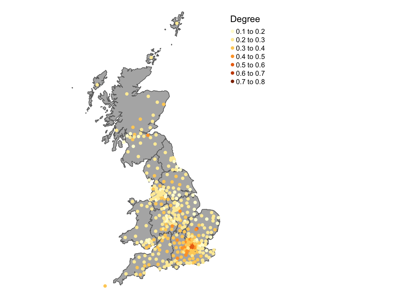

Figure 2.10: Point data values using choropleth mapping (colour).

You should explore the introductory tmap vignettes which describes other approaches for mapping different types of variables, in built styles, plotting multiple layers:

vignette("tmap-getstarted", package = "tmap")

It is possible to use an OpenStreetMap backdrop for some basic web-mapping with tmap by switching the view from the default mode from plot to view. You need to be on-line and connected to the internet. The code below generates a zoomable web-map map with an OpenStreetMap backdrop in the figure below, with a transparency term to aid the understanding of the local map context:

# set the mode
tmap_mode("view")
# do the plot
tm_shape(data_gb[data_gb$Region == "East",]) +
    tm_fill(c("share_leave"), palette = "Reds", alpha = 0.6) +
    tm_basemap('OpenStreetMap')

Aerial imagery and satellite imagery (depending on the scale and extent of the scene) can also be used to provide context as in the figure below:

tm_shape(data_gb[data_gb$Region == "East",]) +
    tm_fill(c("share_leave"), palette = "Reds", alpha = 0.6) +
    tm_basemap('Esri.WorldImagery')

Other backdrops can be specified as well as OSM. Try the following: Stamen.Watercolor, Esri.WorldGrayCanvas, OpenStreetMap and Esri.WorldTopoMap.

The tmap_mode needs to be reset to return to a normal map view:

tmap_mode("plot")

Finally in this brief description of tmap, when maps are assigned to a named R object (like p1) then you can exert greater control over how multiple maps are plotted together using the tmap_arrange function. This allows the parameters for each map to be specified individually before they displayed together as in the figure below.

p1 <- tm_shape(data_gb) + 
  tm_fill("younger_adults", palette = "Reds", style = "quantile", 
          n = 5, title = "Younger Adults")+
  tm_layout(legend.position = c("left", "top"))+
  tm_shape(regions) + tm_borders(col = "black", lwd = 1)
p2 <- tm_shape(data_gb) + 
  tm_fill("private_transport_to_work", palette = "YlGn", style = "quantile", 
          n = 5, title = "Car Commute")+
  tm_layout(legend.position = c("left", "top"))+
  tm_shape(regions) + tm_borders(col = "black", lwd = 1)
p3 <- tm_shape(data_gb) + 
  tm_fill("not_good_health", palette = "YlOrRd", style = "quantile", 
          n = 5, title = "Poor health")+
  tm_layout(legend.position = c("left", "top"))+
  tm_shape(regions) + tm_borders(col = "black", lwd = 1)
tmap_arrange(p1,p2,p3, nrow = 1)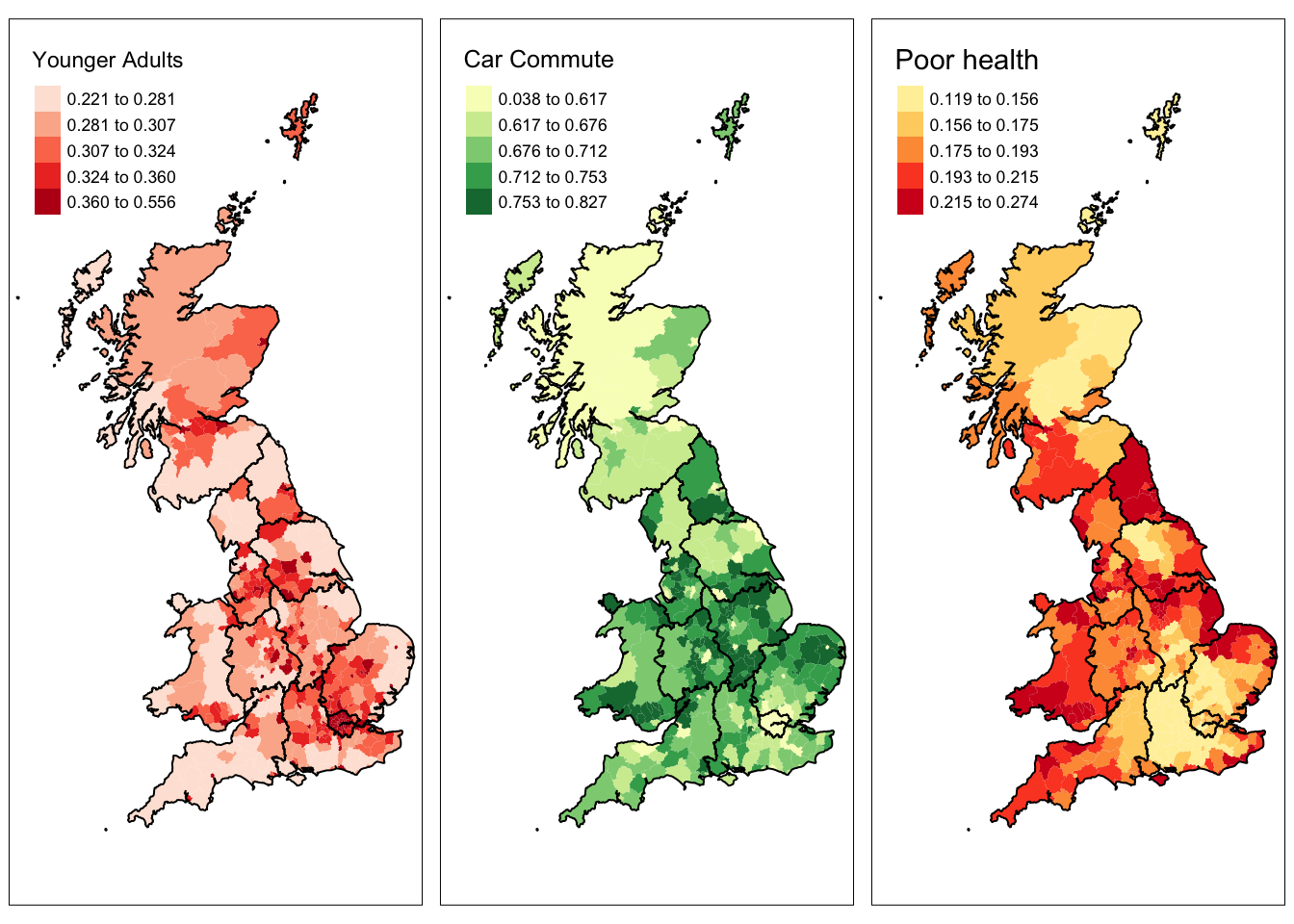

(#fig:ch2fig16,)The result of combining multiple tmap objects.

The full functionality of tmap has only been touched on. It is covered in much greater depth throughout in Brunsdon and Comber (2018) but particularly in Chapters 3 and 5.

Key Points:

The basic syntax for mapping using the tmap package was introduced;
This has a layered form tm_shape(data = <data>) + tm_<function>()
By default tmap allocates a colour scheme, decides the breaks (divisions) for the attribute being mapped, places the legend somewhere, gives a legend title etc. All of these can be changed;
Additional spatial data layers can be added to the map;
tmap has all the usual map embellishments (scale bar, north arrow etc);
tmap allows interactive maps to be created with different map backdrops (e.g. OpenStreetMap, aerial imagery, etc);
the tmap_arrange function allows multiple maps to plotted together in the same plot window.

2.5 Useful Resources

There are few links in the list below that you may find useful:

Spatial operations, Chapter 4 in https://geocompr.robinlovelace.net/spatial-operations.html
An Intro to Spatial Data Analysis https://www.spatialanalysisonline.com/An%20Introduction%20to%20Spatial%20Data%20Analysis%20in%20R.pdf
Making Maps with R https://bookdown.org/nicohahn/making_maps_with_r5/docs/introduction.html
Chapter 5 in https://geocompr.robinlovelace.net/adv-map.html
An Introduction to Spatial Data Analysis and Visualisation in R https://data.cdrc.ac.uk/dataset/introduction-spatial-data-analysis-and-visualisation-r

Data sources also:

ONS spatial data: https://geoportal.statistics.gov.uk/search?collection=Map
Spatial data from ONS (shapefile format) - https://www.data.gov.uk/search?q=&filters%5Bpublisher%5D=&filters%5Btopic%5D=Mapping&filters%5Bformat%5D=SHP&sort=best
House of Commons data: https://commonslibrary.parliament.uk/data-tools-and-resources/
uk-hex-cartograms-noncontiguous, House of Commons github, https://github.com/houseofcommonslibrary/uk-hex-cartograms-noncontiguous
the parlitools package has lots of voting data https://cran.r-project.org/web/packages/parlitools/vignettes/introduction.html

References

Beecham, Roger, Nick Williams, and Alexis Comber. 2020. “Regionally-Structured Explanations Behind Area-Level Populism: An Update to Recent Ecological Analyses.” Plos One 15 (3): e0229974.

Brunsdon, Chris, and Lex Comber. 2018. An Introduction to r for Spatial Analysis and Mapping (2e). Sage.

Comber, Lex, and Chris Brunsdon. 2021. Geographical Data Science and Spatial Data Analysis: An Introduction in r. Sage.

Chapter 2 Data and spatial data in R

2.1 Introduction

2.1.1 Packages

2.1.2 Data

2.2 Using R as a GIS

2.2.1 Creating point data

2.2.2 Spatial Operations

2.2.3 Merging spatial features and Buffers

2.2.4 Point-in-polygon and Area calculations

2.2.4.1 Point-in-polygon

2.2.4.2 Area calculations

2.2.5 Creating distance attributes

2.2.6 Reading and writing data in and out of R/RStudio

2.3 Answer to Tasks

2.4 Optional: mapping with tmap

2.4.1 Mapping with tmap

2.5 Useful Resources

References

2.4 Optional: mapping with `tmap`

2.4.1 Mapping with `tmap`