Chapter 7 Introduction to Analysis of Variance (ANOVA)

by Heather Kropp for ENVST 206: Introduction to Environmental Data Hamilton College

7.1 Learning objectives

Work with data related to measures of biodiversity
Learn to conduct an ANOVA in R
Visualize and interpret an ANOVA

7.2 New functions & syntax

aov, TukeyHSD

7.3 Measuring biodiversity: the data

A decline in biodiversity is a common environmental concern. Biodiversity is a concept related to a wide range in the number of species (plant, fungi, and animal) and abundance of populations in a species. Anthropogenic impacts on the environment via habitat loss, increased global temperatures, and pollution can all negatively impact the abundance of living organisms. Extinction of organisms as a result of these impacts is decreasing biodiversity. There are a number of ways to measure biodiversity. Species richness is the number of different types of species present in a particular location. It is typically measured as a numerical count of species and collected from observations that look for presence/absence of different species. Diversity indices account for both the number of different types of species and the evenness of the number of individuals in each type of species.

The urban environment can affect survival and reproduction of some insect species. Built environments are warmer environments with less water availability, particularly in drier regions of California. Residential areas of urban environments can provide more vegetated environments, but plant cover is often not native and mostly dominated by a single plant cover such as grass. Some insects are not well equipped to survive in many urban environments and there is a concern that urbanization can drive declines in the diversity of insects. This may negatively impact essential part of ecosystems driving pollination, the food web, and the decomposition of plant material.

To evaluate the impact of the urban environment on insects, Adams et al. (2019) trapped insects across the Los Angeles area and examined the number of species at each location. Below is a map of sampling locations used in the study across differing levels of urbanization.

Aerial view of Los Angeles area highlights the varying levels of urbanization from the highly devleoped areas of commercial complexes and downtown to mountain parks Source: Tuxyso, CC BY-SA 3.0, via Wikimedia Commons

#read in insect data
datI <- read.csv("/cloud/project/activity06/insect_richness.csv")

  urbanType urbanName Richness lawn
1         3  Suburban       30  Yes
2         8 Developed        3  Yes
3         9     Dense       22   No
4         9     Dense        1  Yes
5         8 Developed       22   No
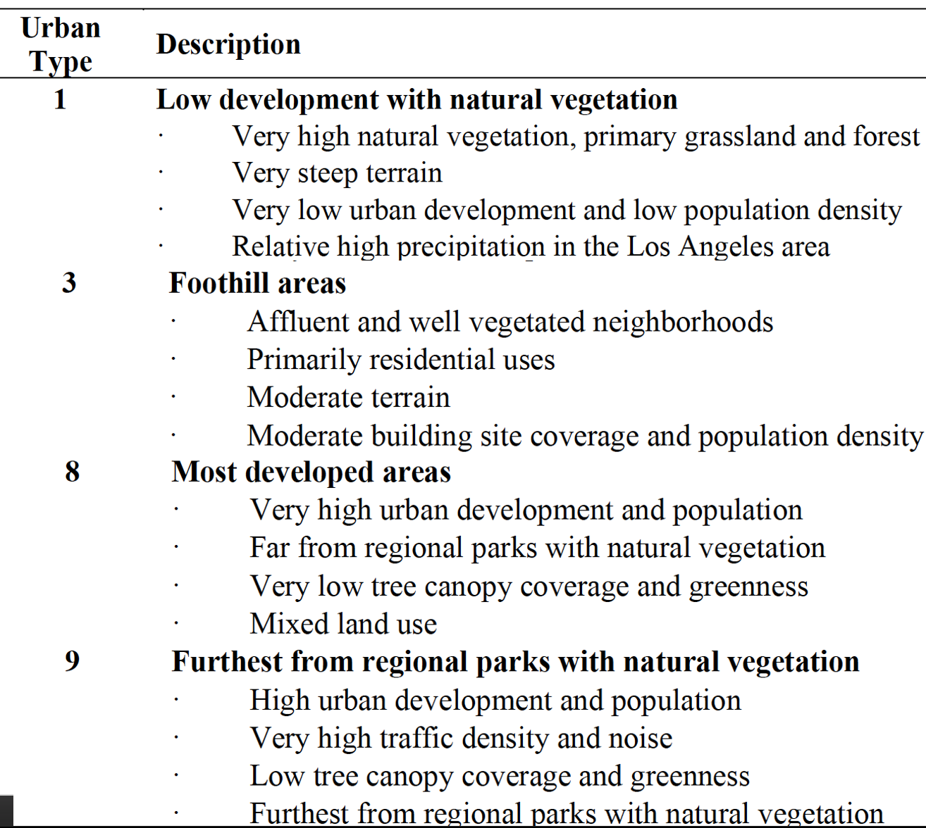
6         8 Developed       15   No

As you learned in class, ANOVA is a widely used technique for testing for differences in three or more groups. ANOVA will be useful for examining the insect species richness across an urban gradient in Los Angles. The Richness and the urbanName column will be used for the test. urbanName gives the type of urban environment the species richness was measured in. You will want to specify urbanName as a factor to work best in the ANOVA. The urbanType column provides an identifying number originally used in by the authors. We are only focusing on a few urban areas in this analysis. Below is a table that provides a more detailed description of each area used in the study site. The numbers in the table coincide with the urbanType column.

_Table describing urban type classification from Adams et al. (2019)

It will be helpful to convert the names to factors in R.

datI$urbanName <- as.factor(datI$urbanName)

7.4 ANOVA overview

In ANOVA, the F-ratio is a statistic that is used to evaluate differences in data between groups. First the among group (SS_among, sometimes referred to as between) sum of squares calculates the squared difference between each group mean and the overall mean of all the data and sums up the differences for all groups. The within group (SS_within, also referred to as residual) sum of squares calculates the squared difference between each data observation and its group mean and sums these differences for all observations. The mean squares is then calculated using the number of groups (SS_among) and both the number of groups and observations (SS_within). The F-ratio is calculated by dividing the mean square for among groups by within groups (see table below). The p-value provides a probability for observing the calculated F-ratio and all values higher than the ratio. For this class, we can assume the confidence level of 0.05 to make your assessment.

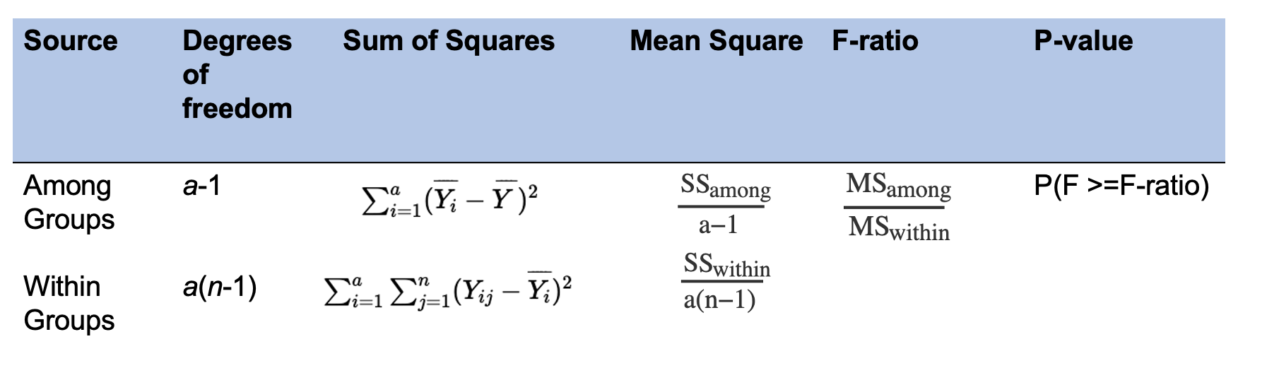
Here a represents the total number of groups and n represents the number of observations within groups.

7.5 ANOVA in R

7.5.1 Checking assumptions

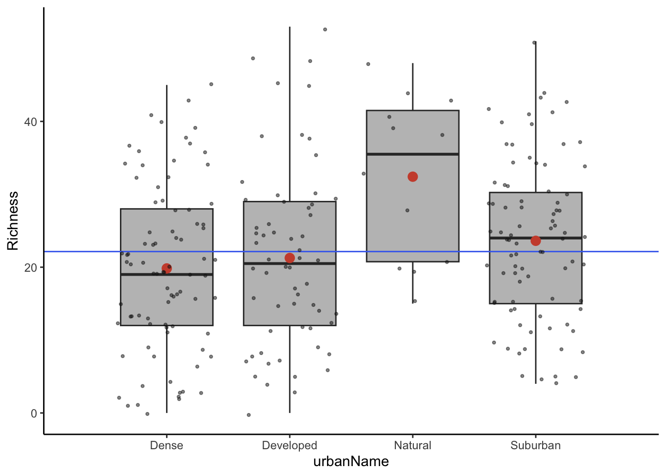
Next you will run the ANOVA test on the insect data to examine whether the different urban environments impact species richness. Before checking the assumptions, it’s a good idea to visualize the data. I’ll show the data using the plots from class that help visualize the different values used in ANOVA. The grey points show individual observations overlain on the boxplot for each group. The red points show the group mean and the blue line shows the mean for all the data.

The first assumption is normality for each group. You must check normality for each individual group. Don’t forget that unique can be helpful for getting the names for each group:

unique(datI$urbanName)

[1] Suburban  Developed Dense     Natural  
Levels: Dense Developed Natural Suburban

The sample size is small enough to use the Shapiro Wilk’s test.


    Shapiro-Wilk normality test

data:  datI$Richness[datI$urbanName == "Suburban"]
W = 0.98087, p-value = 0.2461


    Shapiro-Wilk normality test

data:  datI$Richness[datI$urbanName == "Developed"]
W = 0.96155, p-value = 0.05604


    Shapiro-Wilk normality test

data:  datI$Richness[datI$urbanName == "Dense"]
W = 0.97508, p-value = 0.1025


    Shapiro-Wilk normality test

data:  datI$Richness[datI$urbanName == "Natural"]
W = 0.91559, p-value = 0.2514

The null hypothesis is that the data are normally distributed. Here, each group is higher than our confidencle level of 0.05.

The second assumption of equal variance can be checked with the Bartlett test.

bartlett.test(datI$Richness~datI$urbanName)


    Bartlett test of homogeneity of variances

data:  datI$Richness by datI$urbanName
Bartlett's K-squared = 1.2091, df = 3, p-value = 0.7508

Both equal variance and normality assumptions are appropriate for the data. The other assumptions are that observations are independent of each other and correctly classified in each group. Since this data comes from a peer reviewed study that also uses frequentist statistics, we can assume that the research design and data are set up to meet these assumptions.

7.5.2 Running the ANOVA

Now that you’ve had a chance to check the assumptions and visualize the data, you are ready to run the ANOVA in R. There are two steps to this test in R. You first specify a linear model with the lm function. The next step is to run the ANOVA calculations using aov function. Both of these functions will simply run the calculations. To view the ANOVA table of results, you will print the table using the summary function. In the lm function we will specify a formula Richness ~ Urban.

#specify model for species richness and urban type
in.mod <- lm(datI$Richness ~ datI$urbanName)
#run the ANOVA
in.aov <- aov(in.mod)
#print out ANOVA table
summary(in.aov)

                Df Sum Sq Mean Sq F value  Pr(>F)   
datI$urbanName   3   1944   647.9   4.898 0.00254 **
Residuals      236  31216   132.3                   
---
Signif. codes:  0 '***' 0.001 '**' 0.01 '*' 0.05 '.' 0.1 ' ' 1

Here the table will print out such that the upper row labeled with our group vector name (datI$urbanName) is our among group variability (sum of squares for group means compared to overall mean) and the residuals row is the within group variability. You can see the F value in the upper right part of the table and the associated p-value.

7.5.3 Post hoc comparisons

The ANOVA results alone do not give us a complete picture of the differences between urban landcover types. Some groups actually look quite similar. You must check to see how the means compare between groups to make a full statistical conclusion. You would want to highlight that only some groups may differ from each other when drawing conclusions about the urban environment impacts on species richness. This pairwise comparison between groups is called a post hoc test. Tukey’s HSD (Honestly Significant Difference) test can be used to conduct this comparison.There is a simple built in function in R. You just have to give the name of the variable that has the ANOVA results.

#run Tukey HSD
tukeyT <- TukeyHSD(in.aov)
#view results
tukeyT

  Tukey multiple comparisons of means
    95% family-wise confidence level

Fit: aov(formula = in.mod)

$`datI$urbanName`
                        diff         lwr        upr     p adj
Developed-Dense     1.433333  -3.5966663  6.4633329 0.8819569
Natural-Dense      12.583333   3.3998525 21.7668141 0.0026479
Suburban-Dense      3.785714  -0.8060261  8.3774547 0.1456297
Natural-Developed  11.150000   1.7397324 20.5602676 0.0128693
Suburban-Developed  2.352381  -2.6776186  7.3823805 0.6210733
Suburban-Natural   -8.797619 -17.9810999  0.3858618 0.0658910

Here you will notice that there are two group names in each row indicating which groups are being compared. A significant difference between groups is indicated when the confidence interval for the difference between the means does not overlap with zero. The p-value will also be below our confidence level threshold of 0.05. Note that this test prints a p-adj value. This means it has made some adjustments to account for the fact that were a comparing many means and should account for this in our calculations.

You can also use the plot function and input the entire test variable to generate a plot that shows the confidence levels for the mean comparisons. This can help you get a better visualization for how close these intervals are to zero since there are a lot of numbers printed out in the table.

#make a plot
#make axes labels smaller than usual to fit on plot using cex.axis 
plot(tukeyT, cex.axis=0.75)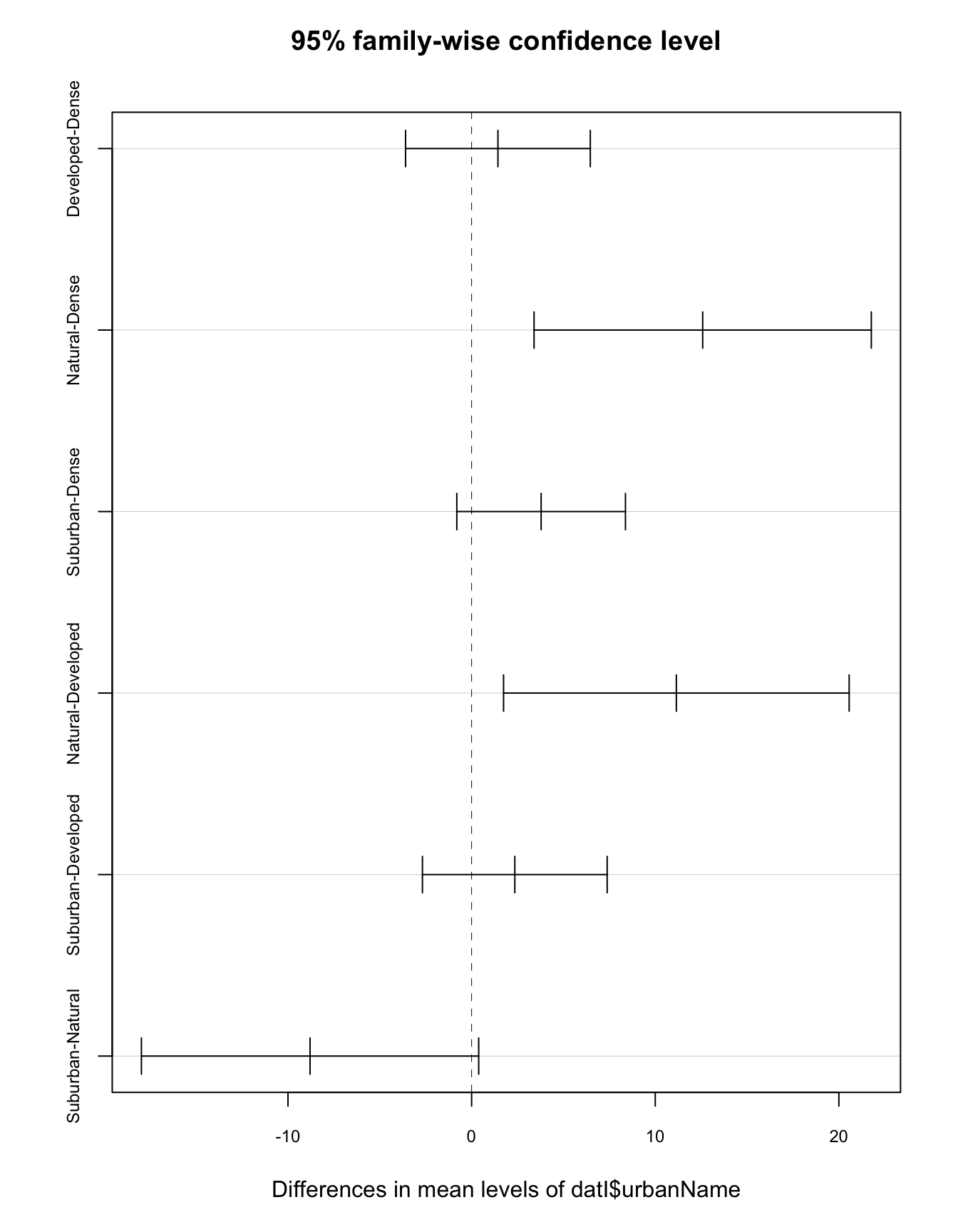

7.5.4 Interpreting the results

When you interpret ANOVA results, you will want to summarize the test results, the means and difference between means, and make a plot that visualizes the data in each group.

Typically a bar or box plot is used to show the means or quartiles of each group with letters above the data to indicate when groups are similar. For example, an ANOVA with four groups that all significantly differed from each other would show a different letter for each group like a,b,c,d.

The Tukey HSD results indicate that the Dense, Developed, and Suburban are all similar. Natural differs from Dense and Developed, but not Suburban. Multiple letters can be used for a group. Dense, Developed, and Suburban all get the letter a. Natural will get the letter b. Since Suburban is similar to Natural, it will also get a b.

The best way to add labels to a base plot in R is the the text function. The arguments are text(x coordinates, y coordinates, text labels to add). In the code below, the coordinates and labels will be set up as vectors.

# box plot
plot(datI$Richness ~ datI$urbanName, 
     xlab = "Urban surface",
     ylab= "Insect species Richness",
     ylim=c(0,60))
# x coordinates for labels
xname <- as.factor(c("Dense","Developed","Natural","Suburban"))
# y coordinates for labels
ylabel <- c(50,55,50,55)
# labels to add
textName <- c("a","a","b","a,b")
# add letters to existing plot
text(xname, #x coordinate
     ylabel, #y coordinate
     textName) # labels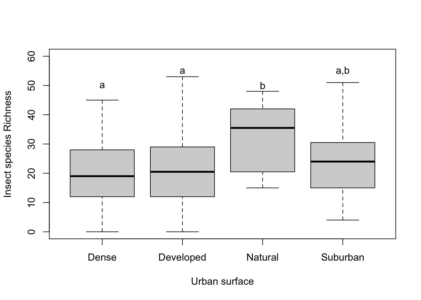

7.6 Citations

Insect Species Richness Adams, B., E. Li, C. Bahlai, E. Meineke, T. McGlynn, and B. Brown. (2020). Local- and landscape-scale variables shape insect diversity in an urban biodiversity hot spot. Ecological Applications. 30: e02089.

Data citation Adams, Benjamin et al. (2020), Local and landscape scale variables shape insect diversity in an urban biodiversity hotspot., v2, Dryad, Dataset, https://doi.org/10.5061/dryad.7d7wm37rd

output: html_document: theme: yeti highlight: pygments —