HW2
2021-03-17
Chapter 1 Prerequisites
This is a sample book written in Markdown. You can use anything that Pandoc’s Markdown supports, e.g., a math equation \(a^2 + b^2 = c^2\).
The bookdown package can be installed from CRAN or Github:
install.packages("bookdown")
# or the development version
# devtools::install_github("rstudio/bookdown")
Remember each Rmd file contains one and only one chapter, and a chapter is defined by the first-level heading #.
To compile this example to PDF, you need XeLaTeX. You are recommended to install TinyTeX (which includes XeLaTeX): https://yihui.name/tinytex/.
# Code chunk 1 for HW1
# head() is a function in base-R that display only the first 6 observations
head(iris)
## Sepal.Length Sepal.Width Petal.Length Petal.Width Species
## 1 5.1 3.5 1.4 0.2 setosa
## 2 4.9 3.0 1.4 0.2 setosa
## 3 4.7 3.2 1.3 0.2 setosa
## 4 4.6 3.1 1.5 0.2 setosa
## 5 5.0 3.6 1.4 0.2 setosa
## 6 5.4 3.9 1.7 0.4 setosa# Code chunk 2 for HW1
# tidying the raw data into the tidy data using `pivot_longer()` and `separate()` functions in the tidyr package
library(tidyverse)## Warning: package 'tidyverse' was built under R version 4.0.4## -- Attaching packages ------------------------- tidyverse 1.3.0 --## √ ggplot2 3.3.3 √ purrr 0.3.4
## √ tibble 3.0.6 √ dplyr 1.0.4
## √ tidyr 1.1.2 √ stringr 1.4.0
## √ readr 1.4.0 √ forcats 0.5.1## Warning: package 'readr' was built under R version 4.0.4## Warning: package 'forcats' was built under R version 4.0.4## -- Conflicts ---------------------------- tidyverse_conflicts() --
## x dplyr::filter() masks stats::filter()
## x dplyr::lag() masks stats::lag()iris %>%
pivot_longer(cols = -Species, names_to = "Part", values_to = "Value") %>%
separate(col = "Part", into = c("Part", "Measure"))## # A tibble: 600 x 4
## Species Part Measure Value
## <fct> <chr> <chr> <dbl>
## 1 setosa Sepal Length 5.1
## 2 setosa Sepal Width 3.5
## 3 setosa Petal Length 1.4
## 4 setosa Petal Width 0.2
## 5 setosa Sepal Length 4.9
## 6 setosa Sepal Width 3
## 7 setosa Petal Length 1.4
## 8 setosa Petal Width 0.2
## 9 setosa Sepal Length 4.7
## 10 setosa Sepal Width 3.2
## # ... with 590 more rows# Code chunk 3 for HW1
# transforming our data using `group_by()` and `summarize()` functions in the dplyr package
# Because we created the `Part` variable in our tidy data,
# we can easily calculate the mean of the `Value` by `Species` and `Part`
iris %>%
  pivot_longer(cols = -Species, names_to = "Part", values_to = "Value") %>%
separate(col = "Part", into = c("Part", "Measure")) %>%
group_by(Species, Part) %>%
summarize(m = mean(Value))## # A tibble: 6 x 3
## # Groups: Species [3]
## Species Part m
## <fct> <chr> <dbl>
## 1 setosa Petal 0.854
## 2 setosa Sepal 4.22
## 3 versicolor Petal 2.79
## 4 versicolor Sepal 4.35
## 5 virginica Petal 3.79
## 6 virginica Sepal 4.78# Code chunk 4 for HW1
# visualizing our data using `ggplot()` function in the `ggplot2` package
iris %>%
pivot_longer(cols = -Species, names_to = "Part", values_to = "Value") %>%
separate(col = "Part", into = c("Part", "Measure")) %>%
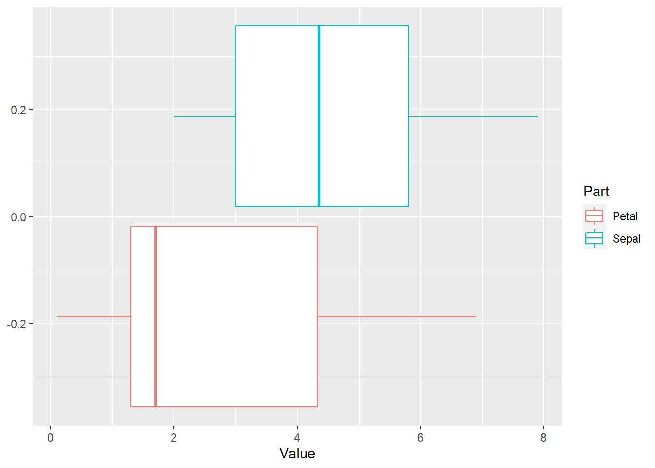
ggplot(aes(x = Value, color = Part)) + geom_boxplot()
bookdown::publish_book(render = ‘local’)