Shiny integration example
2021-07-05
Chapter 1 Inference about a mean

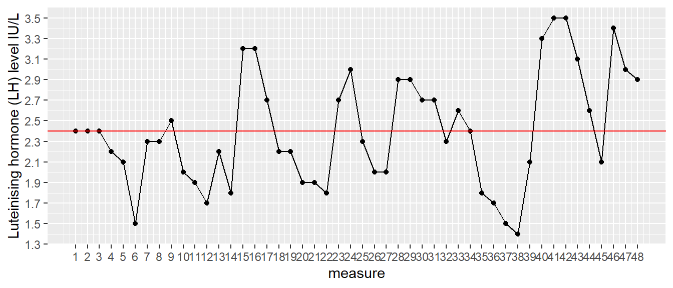
(#fig:mean_data)Luteinising hormone levels measured in one female, 48 measures taken at 10-minute intervals.
1.1 The problem of inference
The human body is heavily controlled by hormones. One of the hormones involved in a healthy reproductive system is luteinising hormone (LH). This hormone is present in both females and males, but with different roles. In females, a sudden rise in LH levels triggers ovulation (the release of an egg from an ovary). We have a data set on luteinising hormone (LH) levels in one anonymous female. The data are given in Figure 2.1. In this data set, we have 48 measures, taken at 10-minute intervals. We see that LH levels show quite some variation over time. Suppose we want to know the mean level of luteinising hormone level in this woman, how could we do that?
The easiest way is to compute the mean of all the values that we see in this graph. If we do that here, we get the value 2.4. That value is displayed as the red line in Figure 2.1. However, is that really the mean of the hormone levels during that time period? The problem is that we only have 48 measures; we do not have information about the hormone levels in between measurements. We see some very large differences between two consecutive measures, which makes the level of hormone look quite unstable. We lack information about hormone levels in between measurements because we do not have data on that. We only have information about hormone levels at the times where we have observed data. For the other times, we have unobserved or missing data.
Suppose that instead of the mean of the observed hormone levels, we want to know the mean of all hormone levels during this time period: not only those that are measured at 10-minute intervals, but also those that are not measured (unobserved/missing).
You could imagine that if we would measure LH not every 10 minutes, but every 5 minutes, we would have more data, and the mean of those measurements would probably be somewhat different than 2.4. Similarly, if we would take measurements every minute, we again would obtain a different mean. Suppose we want to know what the true mean is: the mean that we would get if we would measure LH continuously, that is, an infinite number of measurements. Unfortunately we only have these 48 measures to go on. We would like to infer from these 48 measures, what the mean is of LH level had we measured continuously.
This is the problem of inference: how to infer something about complete data, when you only see a small subset of the data. The problem of statistical inference is when you want to say something about an imagined complete data set, the population, when you only observe a relatively small portion of the data, the sample.
In order to show you how to do that, we do a thought experiment. Imagine a huge data set on African elephants where we measured the height of each elephant currently living (today around 415,000 individuals). Let’s imagine that for this huge data set, the mean and the variance are computed: a mean of 3.25 m and a variance of 0.14 (recall, from Chapter 1, that the variance is a measure of spread, based on the sums of squared differences between values and the mean). We call this data set of all African elephants currently living the population of African elephants.
Now that we know that the actual mean equals 3.25 and the actual variance equals 0.14, what happens if we only observe 10 of these 415,000 elephants? In our thought experiment we randomly pick 10 elephants. Random means that every living elephant has an equal chance of being picked. This random sample of 10 elephants is then used to compute a mean and a variance. Imagine that we do this exercise a lot of times: every time we pick a new random sample of 10 elephants, and you can imagine that each time we get slightly different values for our mean, but also for our variance. This is illustrated in Table 2.1, where we show the data from 5 different samples (in different columns), together with 5 different means and 5 different variances.
What we see from this table is that the 5 sample means vary around the population mean of 3.25, and that the 5 variances vary around the population variance of 0.14. We see that therefore the mean based on only 10 elephants gives a rough approximation of the mean of all elephants: the sample mean gives a rough approximation of the population mean. Sometimes it is too low, sometimes it is too high. The same is true for the variance: the variance based on only 10 elephants is a rough approximation, or estimate, of the variance of all elephants: sometimes it is too low, sometimes it is too high.
% latex table generated in R 4.0.5 by xtable 1.8-4 package % Mon Jul 05 10:22:58 20211.2 Sampling distribution of mean and variance
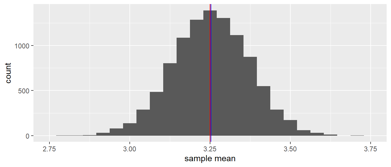
How high and how low the sample mean can be, is seen in Figure 2.2. There you see a histogram of all sample means when you draw 10,000 different samples of each consisting of 10 elephants and for each sample compute the mean. This distribution is a sampling distribution. More specifically, it is the sampling distribution of the sample mean.
The red vertical line indicates the mean of the population data, that is, the mean of 3.25 (the population mean). The blue line indicates the mean of all these sample means together (the mean of the sample means). You see that these lines practically overlap.
What this sampling distribution tells you, is that if you randomly pick 10 elephants from a population, measure their heights, and compute the mean, this mean is on average a good estimate (approximation) of the mean height in the population. The mean height in the population is 3.25, and when you look at the sample means in Figure 2.2, they are generally very close to this value of 3.25. Another thing you may notice from Figure 2.2 is that the sampling distribution of the sample mean looks symmetrical and resembles a normal distribution.

(#fig:mean_mean_distribution_N10)A histogram of 10,000 sample means when the sample size equals 10.

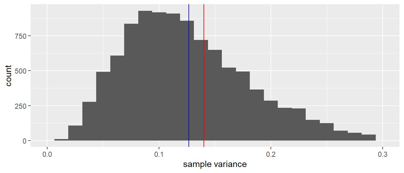
(#fig:mean_var_distribution_N10)A histogram of 10,000 sample variances when the sample size equals 10. The red line indicates the population variance. The blue line indicates the mean of all variances observed in the 10,000 samples.
Now let’s look at the sampling distribution of the sample variance. Thus, every time we randomly pick 10 elephants, we not only compute the mean but also the variance. Figure 2.3 shows the sampling distribution. The red line shows the variance of the height in the population, and the blue line shows the mean variance observed in the 10,000 samples. Clearly, the red and blue line do not overlap: the mean variance in the samples is slightly lower than the actual variance in the population. We say that the sample variance underestimates the population variance a bit. Sometimes we get a sample variance that is lower than the population value, sometimes we get a value that is higher than the population value, but on average we are on the low side.
1.3 The effect of sample size
What we have seen so far is that when the population mean is 3.25 m and we observe only 10 elephants, we may get a value for the sample mean of somewhere around 3.25, but on average, we’re safe to say that the sample mean is a good approximation for the population mean. In statistics, we call the sample mean an unbiased estimator of the population mean, as the expected value (the average value we get when we take a lot of samples) is equal to the population value.
Unfortunately the same could not be said for the variance: the sample variance is not an unbiased estimator for the population variance. We saw that on average, the values for the variances are too low.
Another thing we saw was that the distribution of the sample means
looked symmetrical and close to normal. If we look at the sampling
distribution of the sample variance, this was less symmetrical, see
Figure 2.3. It actually has the shape of
a so-called -(pronounced ‘chi-square’) distribution, which will
be discussed in Chapters 8, 12, 13 and 14. Let’s see what happens when we do not take
samples with 10 elephants each time, but 100 elephants.
Stop and think: What will happen to the sampling distributions of the
mean and the variance? For instance, in what way will Figure
2.2 change when we use 100
elephants instead of 10?
Figure 2.4 shows the sampling
distribution of the sample mean. Again the distribution looks normal,
again the blue and red lines overlap. The only difference with Figure
2.2 is the spread of the
distribution: the values of the sample means are now much closer to the
population value of 3.25 than with a sample size of 10. That means that
if you use 100 elephants instead of 10 elephants to estimate the
population mean, on average you get much closer to the true value!
Now stop for a moment and think: is it logical that the sample means are
much closer to the population mean when you have 100 instead of 10
elephants?
Yes, of course it is, with 100 elephants you have much more information
about elephant heights than with 10 elephants. And if you have more
information, you can make a better approximation (estimation) of the
population mean.
Figure 2.5 shows the sampling distribution of the sample variance. Compared to a sample size of 10, the shape of the distribution now looks more symmetrical and closer to normal. Second, similar to the distribution of the means, there is much less variation in values: all values are now closer to the true value of 0.14. And not only that: it also seems that the bias is less, in that the blue and the red lines are closer to each other.
Here we see three phenomena. The first is that if you have a statistic like a mean or a variance and you compute that statistic on the basis of randomly picked sample data, the distribution of that statistic (i.e., the sampling distribution) will generally look like a normal distribution if sample size is large enough.
It can actually be proven that the distribution of the mean will become a normal distribution if sample size becomes large enough. This phenomenon is known as the Central Limit Theorem. It is true for any population, no matter what distribution it has.[^11] Thus, this means that height in elephants itself does not have to be normally distributed, but the sampling distribution of the sample mean will be normal for large sample sizes (e.g., 100 elephants).
The second phenomenon is that the sample mean is an unbiased estimator of the population mean, but that the variance of the sample data is not an unbiased estimator of the population variance. Let’s denote the variance of the sample data as . Remember from Chapter 1 that the formula for the variance is
We saw that the bias was large for small sample size and small for larger sample size. So somehow we need to correct for sample size. It turns out that the correction is a multiplication with :
where is the corrected estimator of population variance, is the variance observed in the sample, and is sample size. When we rewrite this formula and cancel out , we get a more direct way to compute :
Thus, if we are interested to know the variance or the standard deviation in the population, and we only have sample data, it is better to take the sums of squares and divide by , and not by .
where (pronounced ‘sigma-squared hat’) signifies the estimator of the population variance (the little hat stands for estimator or estimated value).
The third phenomenon is that if sample size increases, the variability of the sample statistic gets smaller and smaller: the values of the sample means and the sample variances get closer to their respective population values. We will delve deeper into this phenomenon in the next section.
(#fig:sampling_distributions)Interactive visualization of sampling distributions for the mean and standard deviation for varying number of samples of varying sizes from a number of different population distributions.
1.4 The standard error
In Chapter 1 we saw that a measure for spread and variability was the variance. In the previous section we saw that with sample size 100, the variability of the sample mean was much lower than with sample size 10. Let’s look at this more closely.
When we look at the sampling distribution in Figure 2.2 with sample size 10, we see that the means lie between 2.8 and 3.71. If we compute the standard deviation of the sample means, we obtain a value of 0.118. This standard deviation of the sample means is technically called the standard error, in this case the standard error of the mean. It is a measure of how uncertain we are about a population mean when we only have sample data to go on. Think about this: why would we associate a large standard error with very little certainty? In this case we have only 10 data points for each sample, and it turns out that the standard error of the mean is a function of both the sample size and the population variance .
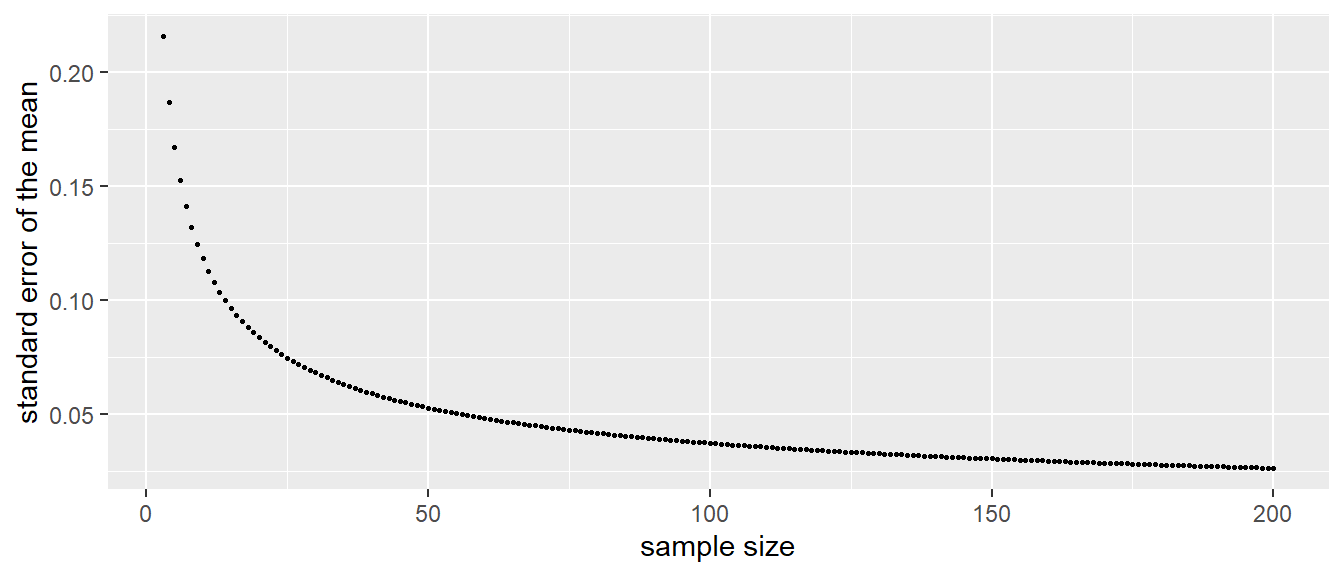
Here, the population variance equals 0.14 and sample size equals 10, so the equals , close to our observed value. If we fill in the formula for a sample size of 100, we obtain a value of 0.037. This is a much smaller value for the spread and this is indeed observed in Figure 2.4. Figure 2.6 shows the standard error of the mean for all sample sizes between 1 and 200.
In sum, the standard error of the mean is the standard deviation of the sample means, and serves as a measure of the uncertainty about the population mean. The larger the sample size, the smaller the standard error, the closer a sample mean is expected to be around the population mean, the more certain we can be about the population mean.
Similar to the standard error of the mean, we can compute the standard error of the variance. This is more complicated – especially if the population distribution is not normal – and we do not treat it here. Software can do the computations for you, and later in this book you will see examples of the standard error of the variance.
Summarising the above: when we have a population mean, we usually see that the sample mean is close to it, especially for large sample sizes. If you do not understand this yet, go back before you continue reading.
The larger the sample size, the closer the sample means are to the population means. If you turn this around, if you don’t know the population mean, you can use a large sample size, calculate the sample mean, and then you have a fairly good estimate for the population. This is useful for our problem of the LH levels, where we have 48 measures. The mean of the 48 measurements could be a good approximation of the mean LH level in general.
As an indication of how close you are to the population mean, the standard error can be used. The standard error of the mean is the standard deviation of the sampling distribution of the sample mean. The smaller the standard error, the more confident you can be that your sample mean is close to the population mean. In the next section, we look at this more closely. If we use our sample mean as our best guess for the population mean, what would be a sensible range of other possible values for the population mean, given the standard error?

(#fig:se_sample_size)Relationship between sample size and the standard error of the mean, when the population variance equals 0.14.