Chapter 2 Preseason Models
In this section, I will outline the process of training a win-prob model at the game level utilizing preseason team variables. I will construct two different models - one to predict score differential and one to predict win probability.
2.1 Score Differential Model
I will first train a model on each game in the past 5 seasons (2014-15 to 2018-19 Season) to come up with an expected score differential between two teams that are playing. Since we are working strictly on predictions made prior to the season starting, we cannot use any performance metrics that the team has (Net Rating, Offensive Net Rating, etc.). In other words, I am confined to using roster variables (Amount of stars on the team, Career Win Share avg. of team, etc.) and location of game (Home/Away) to predict this score differential. To keep things simple, I will train this model within relation to the home team only.
\[\text{Score Diff} = \beta{0}+ \beta1*{\text{OWS Diff.}} + \beta2*{\text{DWS Diff.}} + \beta3*{\text{Roster All-NBA Diff.}} + \epsilon \]
I will gather data for each team for the 2014-15 to 2018-19 NBA seasons to train this model. For Win Share values, I will use each players’ previous 2 season Win Share averages. For All NBA, I will utilize the past seasons All-NBA selections. This data gather is shown in the code chunk below.
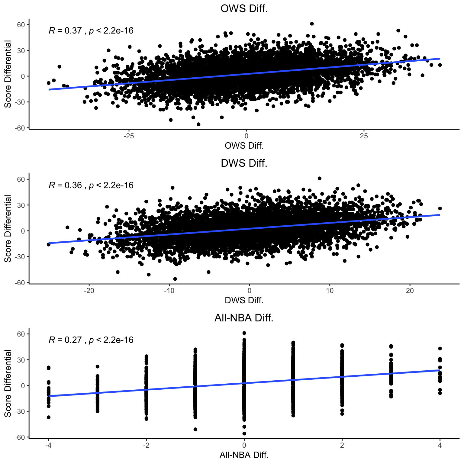
2.1.1 Variable Relationship Plot
We can view general relationships between each independent variable and the score differential for each game in the plot below.
2.1.2 Model Training
We have encouraging variable correlations as shown in the previous plots. Now it is time to train a model to predict score differential of games. I am going to train a model using cv.glmnet from the glmnet package in R.
2.2 Win Prob Model
After training a model to predict score differential, we can then train a model that predicts win probability based on the score prediction. To accomplish this, I utilized a logistic glm modeling technique. The formula that the win-prob model is based on is as follows:
\[\text{Win Probability} = \beta{0}+ \beta1*{\text{Predicted Score Diff.}} + \epsilon \]
To evaluate my win probability model, I also like to create calibration plots as shown below. Here we can see that the model does a good job of predicting game outcomes on both the train data as well as the test dataset.
We now have an accurate win prob model that will be used in our simulations in the following sections.