4 Salt pools
4.1 Introduction
This analysis applies the approach from Naftz (2017) to calculate Gilbert Bay deep brine layer (DBL) & upper brine layer (UBL) volumes and constituent masses to estimate salt masses within Gilbert Bay by brine layer. Data are all from USGS NWIS.
4.2 Objectives
- Estimate Gilbert Bay brine layer salt pools
- Replicate the Naftz (2017) nitrogent pool estimates
- Automate the pool estimate process to allow rapid updates and application to other constituents
4.3 General methods
To estimate salt pools: 1. Estimate monthly UBL and DBL volumes 2. Estimate monthly average brine layer salinities 3. Multiply volumes by salinities to estimate masses
There are two main differences between this analysis and the Naftz approach:
1. I incorporated all available data from all sites in Gilbert Bay in addition to the four monitoring locations used in Naftz (2017).
2. I did not fill missing data by month and site with the previous observed value. Any month with no salinity results available for a brine layer will produce an NA result.
4.3.1 Brine layer volume estimates
Monthly UBL and DBL volumes were estimated from daily Gilbert Bay water surface elevation measurements via surface elevation to DBL elevation and DBL elevation to DBL volume relationships developed as presented in supplementary material 7 from Naftz (2017) and developed by Baskin (2005). These relationships were based on observations from 2010-2014 spanning Gilbert Bay surface water elevations from about 1278-1279 m (~4193-4196 ft). DBL volumes are estimated for north and south DBL basins separately. Note that the model terms presented in Naftz (2017) supplementary material 7 were rounded, so I re-modeled these relationships to generate the surface elevation to volume relationships.
4.3.2 Brine layer salinity estimates
Salinities calculated from density via the GSL equation of state (Naftz et al. 2011) were used to estimate brine layer salinities. I estimated monthly average salinities in each brine layer by averaging all salinity samples collected within each brine layer. Samples were assigned to a brine layer by site location and depth. DBL samples were defined as those occurring at sites 405356112205601 (south) or 410644112382601 (north) and with sampling depth >= 5 meters (see map, 6.1). UBL samples were defined as any sample in Gilbert Bay <= 2 meters sampling depth.
4.3.3 Mass calculations
Salt masses are estimated by multiplying monthly brine layer volumes by monthly average salinities (mass/volume). The north and south DBL basin masses were summed to simplify plots.
4.4 Validation
I validated this mass estimation method against the original Naftz (2017) estimates by comparing monthly values estimated for their target constituent (dissolved nitrogen) from both approaches. Overall, there is strong agreement between the two methods (Figures 4.1 & 4.2).
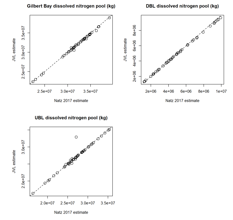
Figure 4.1: Scatter plot comparison of north and south DBL & UBL dissolved nitrogen masses between Naftz 2017 and JVL estimates.
Figure 4.2: Time series comparison of north and south DBL & UBL dissolved nitrogen masses between Naftz 2017 and JVL estimates.
4.5 Code
4.5.1 Calculate UBL & DBL volumes
gb_elev_vol=subset(elevation, site_no==10010000)
gb_elev_vol=within(gb_elev_vol, {
    elev_m=elev_ft/3.28084
    DBL_elev_N=-46.51008+1.03163*elev_m
    DBL_elev_N[DBL_elev_N<1269.43714800001]=1269.43714800001 #Setting minimum possible N DBL elevation at inflection point of formula
    DBL_elev_S=-104.967+1.07643*elev_m
    DBL_elev_S[DBL_elev_S<1270.92582600001]=1270.92582600001 #Setting minimum possible S DBL elevation at inflection point of formula
    DBL_vol_N_m3=59633174862208.5-93949911022.036*DBL_elev_N+37003662.2562751*DBL_elev_N^2
    DBL_vol_S_m3=120180569424473-189400877631.774*DBL_elev_S+74622375.23038100*DBL_elev_S^2
    DBL_vol_total_m3=DBL_vol_S_m3+DBL_vol_N_m3
    UBL_vol_m3=(137054926141519-216113402592.612*elev_m+85193657.0902014*elev_m^2)-DBL_vol_total_m3
    GB_vol_m3=137054926141519-216113402592.612*elev_m+85193657.0902014*elev_m^2
    DBL_vol_acreft=DBL_vol_total_m3*0.000810714
    UBL_vol_acreft=UBL_vol_m3*0.000810714
    GB_vol_acreft=GB_vol_m3*0.000810714
    year=lubridate::year(Date)
    month=lubridate::month(Date)
})

DBLn_vol_YrMo=aggregate(DBL_vol_N_m3~year+month,FUN='mean',gb_elev_vol)
DBLs_vol_YrMo=aggregate(DBL_vol_S_m3~year+month,FUN='mean',gb_elev_vol)
UBL_vol_YrMo=aggregate(UBL_vol_m3~year+month,FUN='mean',gb_elev_vol)
gb_vol_YrMo=merge(UBL_vol_YrMo,DBLn_vol_YrMo,by=c("year","month"))
gb_vol_YrMo=merge(gb_vol_YrMo,DBLs_vol_YrMo,by=c("year","month"))
4.5.2 Create flat wq data
4.5.3 ID WQ samples as UBL or DBL representatives
Defined DBL samples as those occurring at sites 405356112205601 or 410644112382601 and with sampling depth >= 5 meters (see map).
Defined UBL samples as any sample in Gilbert Bay >= 2 meters sampling depth.
4.5.4 Calculate monthly means & SDs for UBL & DBL WQ parameters
4.5.5 Calculate masses
gb_pool_data=merge(gb_vol_YrMo, mon_means)
gb_pool_data=within(gb_pool_data, {
    UBL_mass_kg=UBL_vol_m3*UBL_mean # g/L * m3 * 1000 L / 1 m3 * 1 kg / 1,000,000 mg
    DBL_mass_kg=(DBL_mean_n*DBL_vol_N_m3 + DBL_mean_s*DBL_vol_S_m3)
    tot_mass_kg=DBL_mass_kg+UBL_mass_kg
    UBL_mass_mton=UBL_mass_kg/1000
    DBL_mass_mton=DBL_mass_kg/1000
    tot_mass_mton=tot_mass_kg/1000
    YrMo=as.Date(paste0(year,"-",month,"-01"),format='%Y-%m-%d')
})
4.5.6 Salt mass plot
salt_mass_plot=plot_ly(data=gb_pool_data) %>%
            add_trace(type='scatter', y=~tot_mass_mton, x=~YrMo, mode = 'markers', name='Total', marker = list(symbol=4, color = cols[[6]][[1]],size = 10,line = list(color = cols[[6]][[2]],width = 2))) %>% #, line = list(color = cols[[5]][[2]],width = 2)) %>%
            add_trace(type='scatter', y=~UBL_mass_mton, x=~YrMo, mode = 'markers', name='Upper brine layer', marker = list(color = cols[[5]][[1]],size = 10,line = list(color = cols[[5]][[2]],width = 2))) %>% #,line = list(color = cols[[6]][[2]],width = 2)) %>%
            add_trace(type='scatter', y=~DBL_mass_mton, x=~YrMo, mode = 'markers', name='Deep brine layer', marker = list(symbol=2, color = cols[[2]][[1]],size = 10,line = list(color = cols[[2]][[2]],width = 2))) %>% #, line = list(color = cols[[2]][[2]],width = 2)) %>%
            layout(title = "Gilbert Bay salt pool",
                xaxis = list(title = "", range=c(as.numeric(gauge_date_range[2]-365*10)*86400000,as.numeric(gauge_date_range[2])*86400000)),
                yaxis = list(side = 'left', title = 'Salt mass (metric tons)'),
                legend = list(x = 0.85, y = 1)
            ) %>%
            config(displaylogo = FALSE,
                modeBarButtonsToRemove = c(
                    'sendDataToCloud',
                    'hoverClosestCartesian',
                    'hoverCompareCartesian',
                    'lasso2d',
                    'select2d'
                )
            )
4.6 Results
## Warning: Ignoring 17 observations

## Warning: Ignoring 17 observations
Figure 4.3: Estimated Gilbert Bay salt pools by brine layer.
Prior to breach opening, the total salt pool in Gilbert Bay was relatively stable, with just under 20% of the salt pool accounted for in the DBL when still present. The DBL salt pool mixed into the UBL pool when flow between Gilbert and Gunnison Bays was cut off (Aug 2014 - Dec 2016). A decrease in the Gilbert Bay salt pool is apparent following the opening of the causeway breach.
Although DBL samples are apparent in Gilbert Bay, the mass of salt in the DBL is small due to relatively small volume. Recent lake levels are at the very bottom of the WSE:DBL volume relationship. DBL volume is fixed at minimum values at these lake elevations in this calculation.
4.7 Discussion
Expand the empirical WSE:DBL elevation and volume relationships to other lake elevations as possible.
Characterize error & sampling variability.
Consistency with other salt budget components. Salt pools are based on salinity from density via equation of state.
DBL mass estimate gaps resulting from density to salinity conversion masked values (densities exceeding equation of state calibration).
Consider appropriate platforms for communicating, documenting, and integrating SAC analyses.
References
Baskin, R. L. 2005. Calculation of Area and Volume for the South Part of Great Salt Lake, Utah.
Naftz, D. 2017. Inputs and Internal Cycling of Nitrogen to a Causeway Influenced, Hypersaline Lake, Great Salt Lake, Utah, USA. Aquatic Geochemistry 23:199–216.
Naftz, D., F. Millero, B. Jones, and W. Green. 2011. An Equation of State for Hypersaline Water in Great Salt Lake, Utah, USA. Aquatic Geochemistry 17:809–820.