Chapter 11 Plotting and data visualization
11.1 Dataframe setup for visualization
In this lesson we want to make plots to evaluate the average expression in each sample and its relationship with the age of the mouse. So, to this end, we will be adding a couple of additional columns of information to the metadata data frame that we can utilize for plotting.
Let’s first load the data:
11.1.1 Calculating average expression
Let’s take a closer look at our counts data (rpkm_ordered). Each column represents a sample in our experiment, and each sample has > 36,000 total counts. We want to compute the average value of expression for each sample. Taking this one step at a time, if we just wanted the average expression for Sample 1 we can use the R base function mean():
## [1] 10.2661That is great, but we need to get this information from all 12 samples, so all 12 columns. We want a vector of 12 values that we can add to the metadata data frame. What is the best way to do this?
To get the mean of all the samples in a single line of code the map() family of function is a good option.
11.1.2 The map family of functions
The
map()family of functions is available from thepurrrpackage, which is part of the tidyverse suite of packages. We canmap()functions to execute some task/function on every element in a vector, or every column in a dataframe, or every component of a list, and so on.
map()creates a list.map_lgl()creates a logical vector.map_int()creates an integer vector.map_dbl()creates a “double” or numeric vector.map_chr()creates a character vector.The syntax for the
map()family of functions is:
To obtain mean values for all samples we can use the map_dbl() function which generates a numeric vector.
The output of map_dbl() is a named vector of length 12.
11.1.3 Adding data to metadata
Before we add samplemeans as a new column to metadata, let’s create a vector with the ages of each of the mice in our data set.
# Create a numeric vector with ages. Note that there are 12 elements here

age_in_days <- c(40, 32, 38, 35, 41, 32, 34, 26, 28, 28, 30, 32)
Now, we are ready to combine the metadata data frame with the 2 new vectors to create a new data frame with 5 columns:
# Add the new vectors as the last columns to the metadata
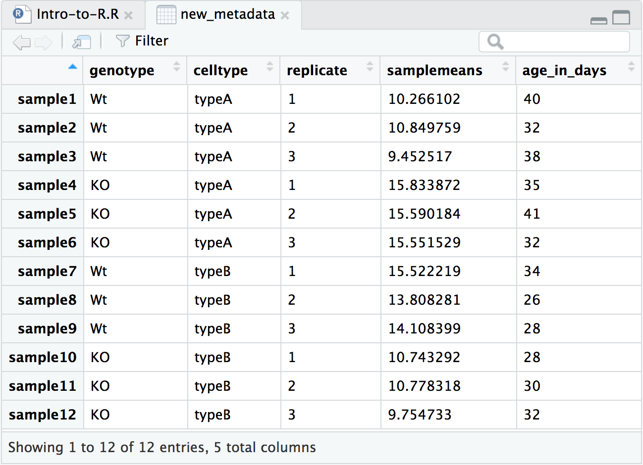
new_metadata <- data.frame(metadata, samplemeans, age_in_days)
# Take a look at the new_metadata object
head(new_metadata)## genotype celltype replicate samplemeans age_in_days
## sample1 Wt typeA 1 10.266102 40
## sample2 Wt typeA 2 10.849759 32
## sample3 Wt typeA 3 9.452517 38
## sample4 KO typeA 1 15.833872 35
## sample5 KO typeA 2 15.590184 41
## sample6 KO typeA 3 15.551529 32Finally, save the new_metadata as a .RData object.
Using new_metadata, we are now ready for plotting and data visualization.