Chapter 5 Negative Binomial model fitting
5.1 Generalized Linear Model fit for each gene
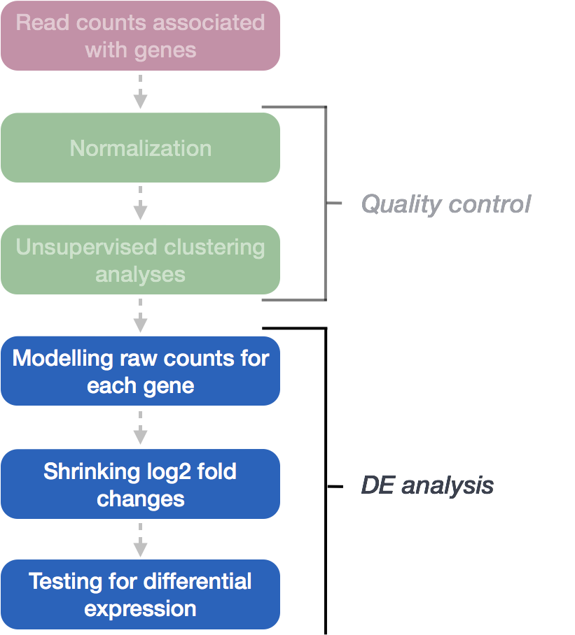
The final step in the DESeq2 workflow is fitting the Negative Binomial (NB) model for each gene and performing differential expression testing. This step is crucial for identifying genes that are significantly differentially expressed between experimental conditions.

DESeq2 uses a Negative Binomial Generalized Linear Model (GLM) to estimate the counts for each gene. A GLM is a statistical method that models relationships between variables and is an extension of linear regression. It is suitable for handling non-normally distributed data, such as RNA-seq counts, which often exhibit overdispersion (variance > mean).
To fit the NB GLM, DESeq2 requires two key parameters:
Size factor, which accounts for differences in sequencing depth across samples.
Dispersion estimate, which measures variability in gene expression across replicates.
The model incorporates the estimated dispersion and the design matrix specifying the experimental conditions and covariates.
5.1.1 Negative Binomial Model Formula
DESeq2 models RNA-seq counts as follows:
Yij∼NB(μij,αi)
Where:
Yij is the observed counts for gene i in sample j
μij is the expected normalized counts for gene i in sample j
αi is the dispersion parameter for gene i, which has been estimated
The expected mean μij is modeled as:
μij=sizeFactorj×qij
Where:
sizeFactorj normalizes for differences in sequencing depth across samples
qij represents the true underlying expression level of gene i in sample j, typically modeled as a function of covariates (such as experimental conditions).
5.1.2 Estimating Beta Coefficients Using the Design Matrix
In DESeq2, beta coefficients (β) are estimated using the design matrix, which captures the experimental conditions for each sample (e.g., control, treatment). These coefficients represent the log2 fold changes in gene expression between different conditions. The estimation process involves fitting a negative binomial generalized linear model (GLM) to the observed count data for each gene, where the expected mean expression μij is modeled as a function of the design matrix Xj and the beta coefficients βi.
5.1.3 Step-by-Step Process:
- Define the Design Matrix Xj:
The design matrix X includes the covariates (experimental conditions) for each sample. Each row of the matrix corresponds to a sample, and each column corresponds to a covariate (e.g., intercept, control, treatment). This matrix is generated using the
model.matrix()function in R.
X <- model.matrix(~ sampletype, data = meta)

# OR

X <- model.matrix(design(dds), data = colData(dds))- Link Mean Expression to the Design Matrix: The expected mean expression for gene i in sample j is modeled as:
log2(μij)=βiXj
Or equivalently:
μij=2βiXj
Here:
Xj is the row of the design matrix for sample j (it contains the covariates for that sample)
βi is the vector of log2 fold changes (beta coefficients) for gene i.
- Estimate the Beta Coefficients: “DESeq2 estimates the beta coefficients by fitting a negative binomial GLM to the data using Maximum Likelihood Estimation (MLE). DESeq2 substitutes the mean (μij) with 2βiXj in the negative binomial model, using MLE to predict expected counts based on experimental covariates and estimate gene expression changes while controlling for design factors.
The model is fit using the DESeq() function in R, which carries out the entire estimation process:
## using pre-existing size factors## estimating dispersions## found already estimated dispersions, replacing these## gene-wise dispersion estimates## mean-dispersion relationship## final dispersion estimates## fitting model and testing- Extract the Beta Coefficients:
Once the model is fitted, the estimated beta coefficients (log2 fold changes) for each gene can be extracted using the
coef()function:
This gives a matrix of estimated beta coefficients, where each row corresponds to a gene and each column corresponds to a covariate in the design matrix.
5.1.4 Example:
For example, if the design matrix includes an intercept (control) and two conditions (MOV10 knockdown and MOV10 overexpression), the beta coefficients βi for gene i would represent:
βi1: the log2 fold change for the control group (intercept)
βi2: the log2 fold change for the MOV10 knockdown group
βi3: the log2 fold change for the MOV10 overexpression group.
5.1.5 Calculation:
To calculate the fitted (expected) log2 counts for gene i in sample j, you can take the dot product of the row of the design matrix Xj for that sample and the beta coefficients βi for that gene:
log2(μij)=βiXj=βi1Xj1+βi2Xj2+⋯+βiPXjP
Where:
- P is the number of covariates in the design matrix
The expected mean μij on the original count scale is obtained by exponentiating the log2-scale fitted values:
μij=2βiXj
Exercise points = +1
In the DESeq2 workflow, what is the purpose of the design matrix in the context of fitting the Negative Binomial model for each gene?
- Ans:
5.1.6 Matrix Multiplication Form:
If you want to calculate the fitted values for all genes and samples at once, you can express the model as a matrix multiplication:
log2(μ)=βXT
This computes the expected log2 counts for all genes across all samples.
In R, you can calculate the fitted log2 counts for all genes and samples using:
This step multiplies the beta coefficients matrix by the transpose of the design matrix to compute the fitted log2 counts.
5.1.7 Log2 Fold Change and Adjustments
The β coefficents are the estimates for the log2 fold changes for each sample group. However, log2 fold changes are inherently noisier when counts are low due to the large dispersion we observe with low read counts. To avoid this, the log2 fold changes calculated by the model need to be adjusted.
5.2 Shrunken log2 foldchanges (LFC)
To generate more accurate LFC estimates, DESeq2 allows for the shrinkage of the LFC estimates toward zero when the information for a gene is low, which could include:
- Low counts
- High dispersion values
As with the shrinkage of dispersion estimates, LFC shrinkage uses information from all genes to generate more accurate estimates. Specifically, the distribution of LFC estimates for all genes is used (as a prior) to shrink the LFC estimates of genes with little information or high dispersion toward more likely (lower) LFC estimates.

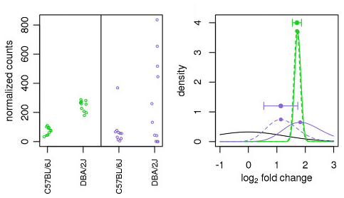
Illustration taken from the DESeq2 paper.
For example, in the figure above, the green gene and purple gene have the same mean values for the two sample groups (C57BL/6J and DBA/2J), but the green gene has little variation while the purple gene has high levels of variation. For the green gene with low variation, the unshrunken LFC estimate (vertex of the green solid line) is very similar to the shrunken LFC estimate (vertex of the green dotted line), but the LFC estimates for the purple gene are quite different due to the high dispersion. So even though two genes can have similar normalized count values, they can have differing degrees of LFC shrinkage. Notice the LFC estimates are shrunken toward the prior (black solid line).
Generating Shrunken LFC Estimates
To generate the shrunken log2 fold change estimates, you have to run an additional step on your results object (that we will create below) with the function lfcShrink()
5.3 Statistical test for LFC estimates: Wald test
In DESeq2, the Wald test is the default used for hypothesis testing when comparing two groups. The Wald test is a test usually performed on the LFC estimates.
DESeq2 implements the Wald test by:
Taking the LFC and dividing it by its standard error, resulting in a z-statistic
The z-statistic is compared to a standard normal distribution, and a p-value is computed reporting the probability that a z-statistic at least as extreme as the observed value would be selected at random
If the p-value is small we reject the null hypothesis (LFC = 0) and state that there is evidence against the null (i.e. the gene is differentially expressed).
5.4 MOV10 Differential Expression Analysis: Control versus Overexpression
We have three sample classes so we can make three possible pairwise comparisons:
- Control vs. Mov10 overexpression
- Control vs. Mov10 knockdown
- Mov10 knockdown vs. Mov10 overexpression
We are really only interested in #1 and #2 from above. Using the design formula we provided ~ sampletype, indicating that this is our main factor of interest.
5.4.1 Creating Contrasts for Hypothesis Testing
In DESeq2, contrasts specify which groups to compare for differential expression testing. You can define contrasts in two ways:
Default Comparison: DESeq2 automatically uses the alphabetically first level of the factor as the baseline.
Manual Specification: You can manually specify the comparison using the
contrastargument in theresults()function. Thecontrastargument takes a vector of three elements. The first element is the name of the factor (design). The second and third elements listed in the contrast are the names of the numerator and denominator level for the fold change, respectively.
Building the Results Table
To build the results table, we use the results() function. You can specify the contrast to be tested using the contrast argument. In this example, we’ll save the unshrunken and shrunken results of Control vs. Mov10 overexpression to different variables. We’ll also set the alpha to 0.05, which is more stringent than the default value of 0.1.
# define contrasts
contrast_oe <- c("sampletype",
                 "MOV10_overexpression",
                 "control")

# extract results table
res_tableOE_unshrunken <- results(dds,
                                  contrast = contrast_oe,
                                  alpha = 0.05)

resultsNames(dds)
## [1] "Intercept" "sampletype_MOV10_knockdown_vs_control"
## [3] "sampletype_MOV10_overexpression_vs_control"# shrink log2 fold changes
res_tableOE <- lfcShrink(dds = dds,
coef = "sampletype_MOV10_overexpression_vs_control",
res = res_tableOE_unshrunken)## using 'apeglm' for LFC shrinkage. If used in published research, please cite:
## Zhu, A., Ibrahim, J.G., Love, M.I. (2018) Heavy-tailed prior distributions for
## sequence count data: removing the noise and preserving large differences.
## Bioinformatics. https://doi.org/10.1093/bioinformatics/bty895The order of the names determines the direction of fold change that is reported. The name provided in the second element is the level that is used as baseline. So for example, if we observe a log2 fold change of -2 this would mean the gene expression is lower in Mov10_oe relative to the control.
5.4.2 MA Plot
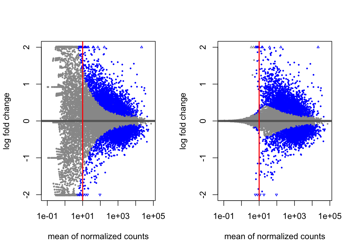
A plot that can be useful to exploring our results is the MA plot. The MA plot shows the mean of the normalized counts versus the log2 foldchanges for all genes tested. The genes that are significantly DE are colored to be easily identified. This is also a great way to illustrate the effect of LFC shrinkage. The DESeq2 package offers a simple function to generate an MA plot.
Shrunken & Unshrunken Results:
par(mfrow = c(1,2))

plotMA(res_tableOE_unshrunken, ylim=c(-2,2))

abline(v = 10,col="red",lwd = 2)

# Shrunken results:
plotMA(res_tableOE, ylim=c(-2,2))

abline(v = 10,col="red",lwd = 2)
MOV10 DE Analysis: Exploring the Results
The results table in DESeq2 looks similar to a data.frame and can be treated like one for accessing or subsetting data. However, it is stored as a DESeqResults object, which is important to keep in mind when working with visualization tools.
## [1] "DESeqResults"
## attr(,"package")
## [1] "DESeq2"
Let’s go through some of the columns in the results table to get a better idea of what we are looking at. To extract information regarding the meaning of each column we can use mcols():
## DataFrame with 5 rows and 2 columns
##                        type            description
##                 <character>            <character>
## baseMean       intermediate mean of normalized c..
## log2FoldChange      results log2 fold change (MA..
## lfcSE               results posterior SD: sample..
## pvalue              results Wald test p-value: s..
## padj                results   BH adjusted p-values
Now let’s take a look at what information is stored in the results:
## log2 fold change (MAP): sampletype MOV10_overexpression vs control
## Wald test p-value: sampletype MOV10 overexpression vs control
## DataFrame with 6 rows and 5 columns
##               baseMean log2FoldChange     lfcSE    pvalue      padj
##              <numeric>      <numeric> <numeric> <numeric> <numeric>
## 1/2-SBSRNA4  45.652040     0.16858121  0.209275 0.1610752 0.2655661
## A1BG         61.093102     0.13623770  0.176713 0.2401909 0.3603094
## A1BG-AS1    175.665807    -0.04016953  0.116916 0.6789312 0.7748342
## A1CF          0.237692     0.00626568  0.210057 0.7945932        NA
## A2LD1        89.617985     0.29007260  0.195380 0.0333343 0.0741149
## A2M 5.860084 -0.09623512 0.233587 0.1057823 0.1900466## [1] "baseMean" "log2FoldChange" "lfcSE" "pvalue" "padj"Interpreting p-values Set to NA
In some cases, p-values or adjusted p-values may be set to NA for a gene. This happens in three scenarios:
Zero counts: If all samples have zero counts for a gene, its baseMean will be zero, and the log2 fold change, p-value, and adjusted p-value will all be set to NA.
Outliers: If a gene has an extreme count outlier, its p-values will be set to NA. These outliers are detected using Cook’s distance.
Low counts: If a gene is filtered out by independent filtering for having a low mean normalized count, only the adjusted p-value will be set to NA.
5.4.3 Multiple Testing Correction
When testing many genes, using raw p-values increases the chance of false positives (genes appearing significant by chance). If we used the p-value directly from the Wald test with a significance cut-off of p < 0.05, that means there is a 5% chance it is a false positives. Each p-value is the result of a single test (single gene). The more genes we test, the more we inflate the false positive rate. This issue is the known as the multiple testing problem. FFor example, if we test 20,000 genes for differential expression, at p < 0.05 we would expect to find 1,000 genes by chance. If we found 3000 genes to be differentially expressed total, 150 of our genes are false positives. We would not want to sift through our “significant” genes to identify which ones are true positives.
DESeq2 addresses this by removing genes with low counts or outliers before testing and by applying the Benjamini-Hochberg (BH) method to control the false discovery rate (FDR).
5.4.4 Benjamini-Hochberg Adjustment
The BH-adjusted p-value is calculated as:
Sort p-values from smallest to largest.
Assign ranks to each p-value pi.
Compute the adjusted p-value:
padji=pi×mi
Where:
pi is the raw p-value
m is the total number of genes tested
i is the rank of the p-value.
Adjusted p-values are compared to a significance threshold (e.g., 0.05) to identify significant genes. The Bonferroni method, another correction, is more conservative and less commonly used due to a higher risk of false negatives.
In most cases, we should use the adjusted p-values (BH-corrected) to identify significant genes.
5.4.5 MOV10 DE Analysis: Control vs. Knockdown
After examining the overexpression results, let’s move on to the comparison between Control vs. Knockdown. We’ll use contrasts in the results() function to extract the results table and store it in the res_tableKD variable. You can also use coef to specify the contrast directly in the lfcShrink() function.
# define contrast
contrast_kd <-  c("sampletype",
                  "MOV10_knockdown",
                  "control")

# extract results table
res_tableKD_unshrunken <- results(dds,
                                  contrast = contrast_kd,
                                  alpha = 0.05)

resultsNames(dds)
## [1] "Intercept" "sampletype_MOV10_knockdown_vs_control"
## [3] "sampletype_MOV10_overexpression_vs_control"# use the `coef` argument to specify the contrast directly
res_tableKD <- lfcShrink(dds, coef = 2,
res = res_tableKD_unshrunken)## using 'apeglm' for LFC shrinkage. If used in published research, please cite:
## Zhu, A., Ibrahim, J.G., Love, M.I. (2018) Heavy-tailed prior distributions for
## sequence count data: removing the noise and preserving large differences.
## Bioinformatics. https://doi.org/10.1093/bioinformatics/bty8955.5 Summarizing Results
To summarize the results, DESeq2 offers the summary() function, which conveniently reports the number of genes that are significantly differentially expressed at a specified threshold (default FDR < 0.05). Note that, even though the output refers to p-values, it actually summarizes the results using adjusted p-values (padj/FDR).
Let’s start by summarizing the results for the OE vs. control comparison:
##
## out of 19748 with nonzero total read count
## adjusted p-value < 0.05
## LFC > 0 (up)       : 3103, 16%
## LFC < 0 (down)     : 3408, 17%
## outliers [1]       : 0, 0%
## low counts [2]     : 4171, 21%
## (mean count < 5)
## [1] see 'cooksCutoff' argument of ?results
## [2] see 'independentFiltering' argument of ?results
In addition to reporting the number of up- and down-regulated genes at the default significance threshold, this function also provides information on:
- Number of genes tested (genes with non-zero total read count)
- Number of genes excluded from multiple test correction due to low mean counts
5.5.1 Extracting Significant Differentially Expressed Genes
In some cases, using only the FDR threshold doesn’t sufficiently reduce the number of significant genes, making it difficult to extract biologically meaningful results. To increase stringency, we can apply an additional fold change threshold.
Although the summary() function doesn’t include an argument for fold change thresholds, we can define our own criteria.
Let’s start by setting the thresholds for both adjusted p-value (FDR < 0.05) and log2 fold change (|log2FC| > 0.58, corresponding to a 1.5-fold change):
Next, we’ll convert the results table to a tibble for easier subsetting:
Now, we can filter the table to retain only the genes that meet the significance and fold change criteria:
sigOE <- res_tableOE_tb %>%
  dplyr::filter(padj < padj.cutoff &
                abs(log2FoldChange) > lfc.cutoff)

# Save the results for future use
saveRDS(sigOE,"data/sigOE.RDS")
Exercise points = +3
How many genes are differentially expressed in the Overexpression vs. Control comparison based on the criteria we just defined? Does this reduce the number of significant genes compared to using only the FDR threshold?
Does this reduce our results?
5.5.2 MOV10 Knockdown Analysis: Control vs. Knockdown
Next, let’s perform the same analysis for the Control vs. Mov10 knockdown comparison. We’ll use the same thresholds for adjusted p-value (FDR < 0.05) and log2 fold change (|log2FC| > 0.58).
res_tableKD_tb <- res_tableKD %>%
  data.frame() %>%
  rownames_to_column(var = "gene") %>%
  as_tibble()

sigKD <- res_tableKD_tb %>%
         dplyr::filter(padj < padj.cutoff &
         abs(log2FoldChange) > lfc.cutoff)

# We'll save this object for use in the homework
saveRDS(sigKD,"data/sigKD.RDS")
How many genes are differentially expressed in the Knockdown compared to Control?
With our subset of significant genes identified, we can now proceed to visualize the results and explore patterns of differential expression.