Multiple Imputation
Background
Multiple imputation is highly recommended as a valid method for handling missing data. It eliminates the disadvantages of reduction in statistical power and under estimation of standard errors when single imputation techniques are applied. Analysis using multiple imputation can be implemented by the following steps:
Step 1: Imputation Missing values are imputed m times (m > 1), resulting in m complete data sets.
Step 2: Analysis Each of these datasets is analyzed using the statistical model chosen to answer the research question. Thus, creating m set of estimates of interest.
Step 3: Pooling The m analysis results(estimates) are combined to one MI result(estimate).
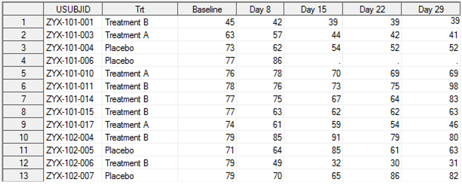
Example data
Consider the following data from a randomized study having three treatment groups – Treatment A, Treatment B and Placebo. PANSS (Positive and Negative Syndrome Scale) was used to assess the effectiveness of the treatment groups in comparison to Placebo. The assessment was repeated on Day 8, 15, 22 and 29 following the initial intake of the study drug. For reducing the effects of missing data, Multiple Imputation is used.
SAS Code
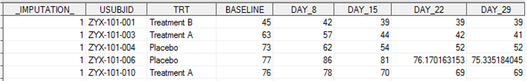
Step 1: Imputation
PROC MI is used for imputing 15 complete sets.
proc mi data = panss_tr out = panssmi seed = 27111433 nimpute = 15 noprint;
  min = . 30 30 30 30 max = . 210 210 210 210;
  class trt;
  var trt baseline day_8 day_15 day_22 day_29;
  fcs reg(/details);
run;
seed specifies a positive integer to begin the random number generation. It is recommended to specify the seed if we’ve to duplicate the results in similar situations or reproduce the results in the future.
nimpute specifies the number of imputations to be performed.
min, max options provide a range of values among which the substituted value for a missing point.
var specifies the variables.
fcs statement specifies an imputation based on fully conditional specification methods.
reg option specifies the regression methods. Since we have not specified any model, SAS constructs the model by using the variables specified in var statement.
details option displays the regression coefficients in each imputation.
Step 2: Analysis
For each of the 15 imputations, ANCOVA model is fitted using PROC MIXED with the fixed, categorical effects of treatment, and the continuous, fixed covariate of Baseline PANSS Total Score. Least square means with corresponding Standard error is estimated for each treatment group.
data panss_mi;
  set panssmi;
  chg = day_29 - baseline;\*change from baseline at Day 29;
run;

proc mixed data = panss_mi;
  by *imputation*;
  class trt;
  model chg = trt baseline;
  lsmeans trt/ cl;
  ods output lsmeans = means;
run;
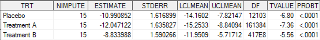
Step 3: Pooling
Estimates are obtained by pooling the analysis results, using the PROC MIANALYZE.
proc sort data = means;
  by trt;
run;

proc mianalyze data = means;
  by trt;
  modeleffects estimate;
  stderr stderr;
  ods output ParameterEstimates = poolestimate;
run;