3 Missingness

3.1 Introduction

When fitting models to a particular data set, missingness is of particular concern. Missing data can lead to biased coefficient estimates. Therefore, a good understanding of the different missingness patterns, their implications on model fitting, and how to deal with them is essential. There are three missingness patterns (missingness mechanisms):

• missingness completely at random (MCAR)
• missingness at random (MAR)
• missingness not at random (MNAR).

In the following sections, we will use a simulated data set containing data on patients and their weight and BMI to illustrate these different mechanisms.

3.2 Missingess Patterns

3.2.1 Simulation Setup

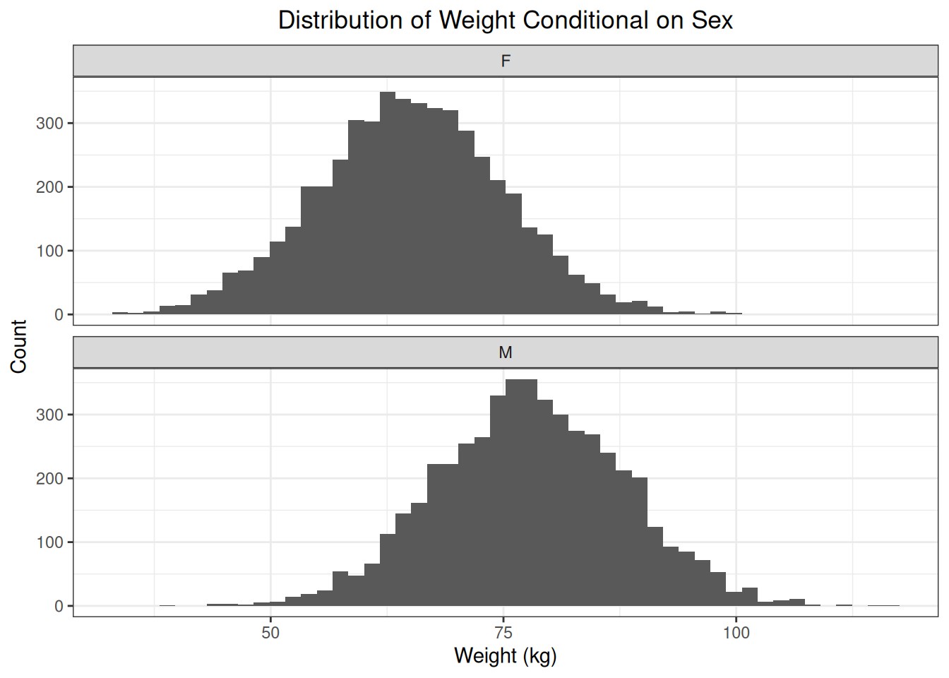
Our simulation setup involves simulating the weight of patients visiting their general physician (GP) for a checkup. For each patient, the sex (male, female) is always recorded. The data set is balanced in terms of sex, and we assume a normally distributed weight (kg) with a mean weight $\mu_{f} = 65$ for women and $\mu_{m} = 78$ for men. The standard deviation $\sigma = 10$ is the same for both sexes:

$$W_{f} \sim \mathcal{N}(65, 100)$$

and

$$W_{m} \sim \mathcal{N}(78, 100).$$

We also simulate the BMI for these patients. We assume the BMI is normally distributed as follows:

$$BMI \sim \mathcal{N}(25, 9).$$

# Simulate patient data. The data set contains 10000 observations, and is 
# balanced in terms of sex.
set.seed(123)
n <- 10000

# Define the parameters that define the distribution of weight and BMI
sd_bmi <- 3
mu_bmi <- 25

sd_weight <- 10
mu_weight_f <- 65
mu_weight_m <- 78

weights <- tibble::tibble(
  idx = 1:n,
  sex = rep(x = c("F", "M"), each = n / 2),
  weight = c(
    rnorm(n / 2, mu_weight_f, sd_weight),
    rnorm(n / 2, mu_weight_m, sd_weight)
  ),
  bmi = round(rnorm(n, mu_bmi, sd_bmi), 1)
)

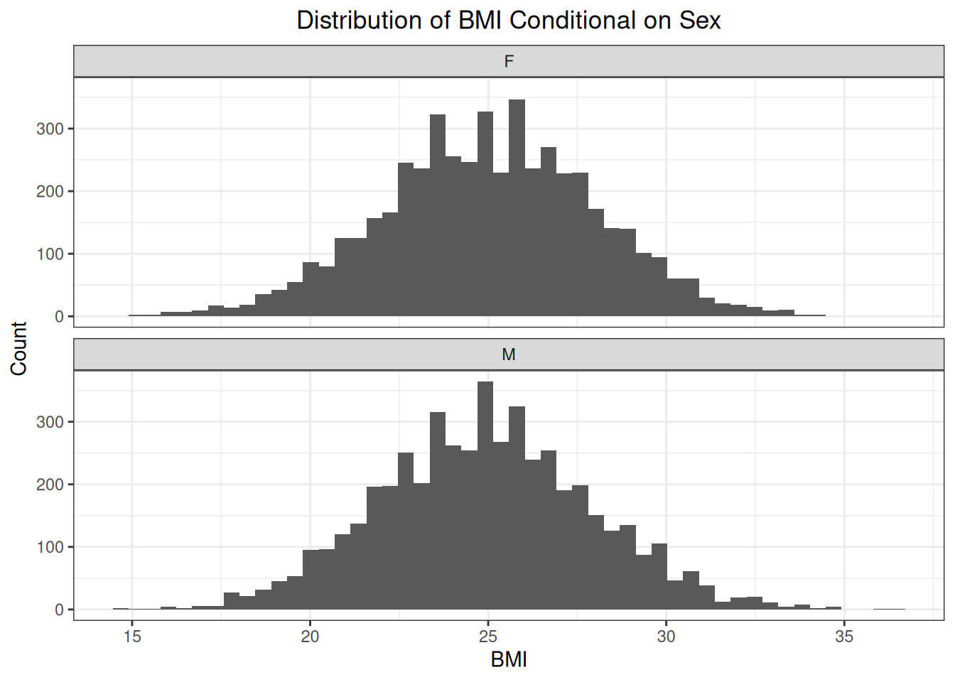
We can see that the conditional distributions of weight given sex have different means.

But the conditional distributions of BMI are the same.

3.2.2 Missingness Completely at Random

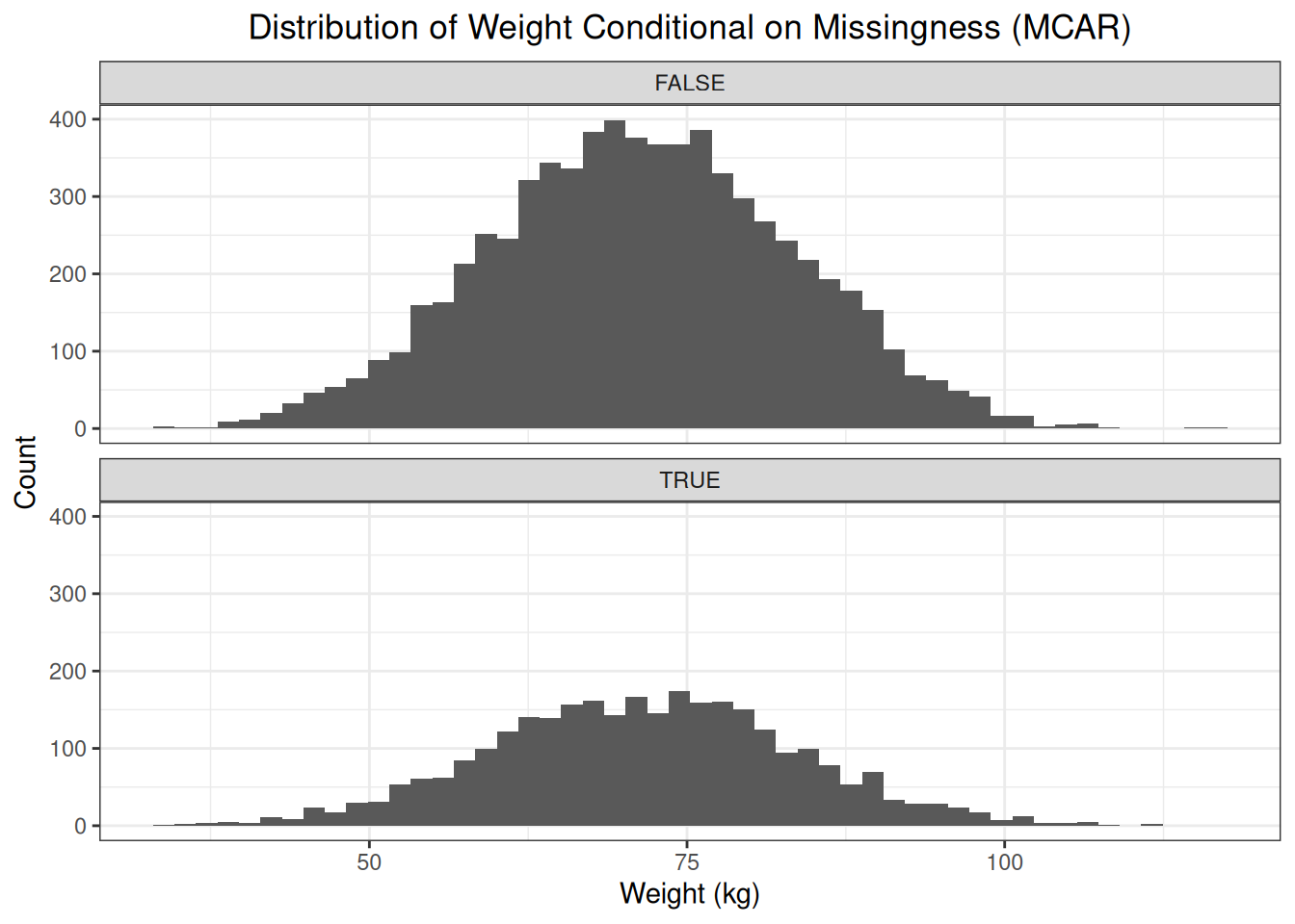
Missingness completely at random indicates that the observations with missing values are a random subset of all observations. There are no factors that affect the probability of missingness, nor is the probability of missingess affected by the outcome itself (weight or BMI). The distribution of observed and missing values is the same.

# Simulate MCAR: assume that 30% of observations have a missing outcome
set.seed(123)
idxs <- sample(x = n, size = n * 0.3)
weights["mcar"] <- weights$idx %in% idxs

Because the observations with missing values are a random subset of all observations, we should see no difference between the distributions of missing and observed values.

3.2.3 Missingness at Random

With missingness at random, we believe there are certain factors that affect the probability of missingness, and that these same factors also have an effect on the outcome. In our example, we see that sex affects the weight. We now assume that sex also affects the probability of missingness.

# Determine the conditional probabilities of missingness
p_missing_f <- 0.45
p_missing_m <- 0.25

idxs <- c(
  sample(
    x = weights[weights$sex == "F", "idx", drop = T],
    size = (n / 2) * p_missing_f
  ),
  sample(
    x = weights[weights$sex == "M", "idx", drop = T],
    size = (n / 2) * p_missing_m
  )
)
weights["mar"] <- weights$idx %in% idxs

Inspection of the distributions of observed and missing values shows us that the distribution of missing values is shifted to the left compared to the distribution of observed values.

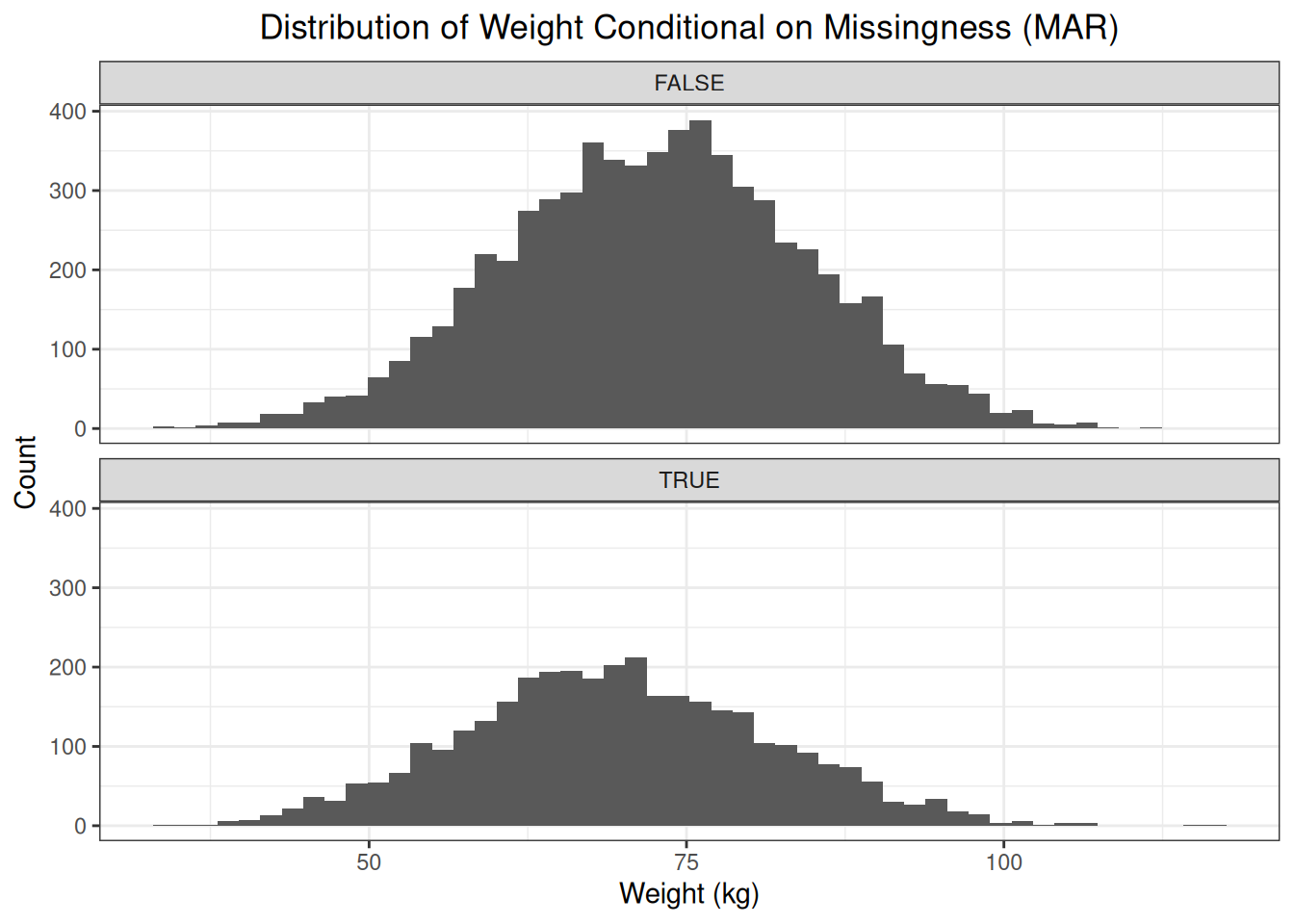
Because the probability of missingness is higher for women then for men, the fraction of patients with a missing weight that are female is higher than the fraction of patients with a missing weight that are men. This affects the distribution of the missing weights, i.e., shifting the distribution to the left. Assume that sex is the only factor that affects the probability of missingness, then, conditional on sex, the distribution of observed values and missing values is the same.

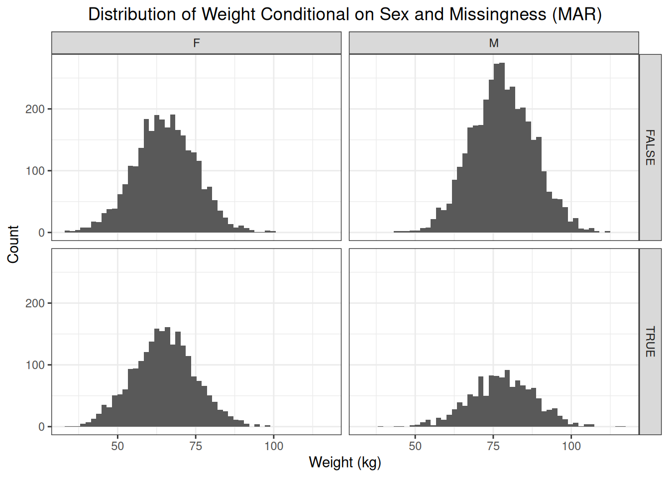
We can see that, conditional on sex, the distribution of observed and missing weights is the same. This illustrates the concept of missingness at random. Sex is the factor that influences both the probability of missingness and the outcome itself. Conditioning on this factors removes the difference in distributions of observed and missing weights.

In practice, it is impossible to conclude missingness at random by comparing the distribution of observed and missing values as the missing values are, of course, missing. This example just demonstrates the concept of missingness at random.

3.2.4 Missingness Not at Random

With missingness not at random, the probability of missingness is not affected by a factor that is recorded, but is affected by factors that are not recorded or even by the outcome itself. For this missingness pattern, we will not focus on the weight of the patient but on the patient’s BMI. The distribution of BMI is the same for women and for men:

However, we could argue the following: if a patient visits the GP, then the GP will more likely weigh the patient if he/she seems overweight or obese. We could make the same argument for underweight patients, but for the sake of illustration, we will assume the likelihood of being weighted is higher for overweight and obese patients. Based on BMI, we can classify patients as:

• underweight: $BMI < 18.5$
• normal: $18.5 \leq BMI \leq 24.9$
• overweight: $25 \leq BMI \leq 29.9$
• obese: $30 \leq BMI$.

We assume the following conditional probabilities of missingness:

# Define conditional probabilities of missingness
p_missing_uw_nw <- 0.75 # underweight and normal weight
p_missing_ow_ob <- 0.55 # overweight and obese

# Classify patients based on their BMI
weights <- weights %>%
  dplyr::mutate(
    bmi_class = dplyr::case_when(
      bmi < 18.5 ~ "uw",
      dplyr::between(bmi, 18.5, 24.9) ~ "nw",
      dplyr::between(bmi, 25.0, 29.9) ~ "ow",
      bmi >= 30.0 ~ "ob"
    )
  )

fd_bmi_classes_df <- weights %>%
  dplyr::group_by(bmi_class) %>%
  dplyr::summarize(n = n())

fd_bmi_classes <- fd_bmi_classes_df$n
names(fd_bmi_classes) <- fd_bmi_classes_df$bmi_class

set.seed(456)

idxs <- c(
  sample(
    x = weights[weights$bmi_class %in% c("uw", "nw"), "idx", drop = T],
    size = round((fd_bmi_classes["uw"] + fd_bmi_classes["nw"]) * p_missing_uw_nw)
  ),
  sample(
    x = weights[weights$bmi_class %in% c("ow", "ob"), "idx", drop = T],
    size = round((fd_bmi_classes["ow"] + fd_bmi_classes["ob"]) * p_missing_ow_ob)
  )
)
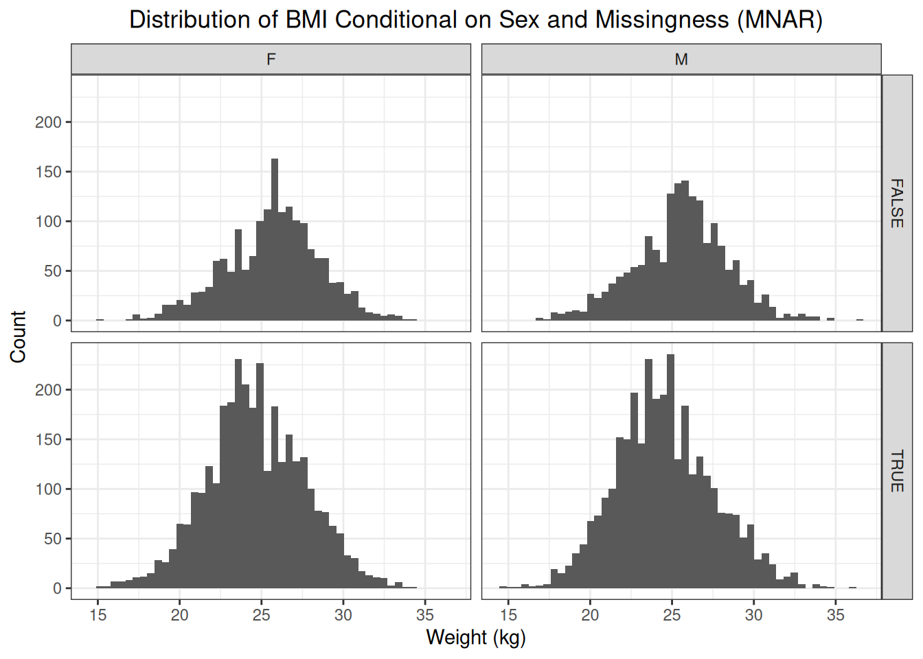
weights["mnar"] <- weights$idx %in% idxs

First, let’s have a look at the distribution of BMI conditional on missingness.

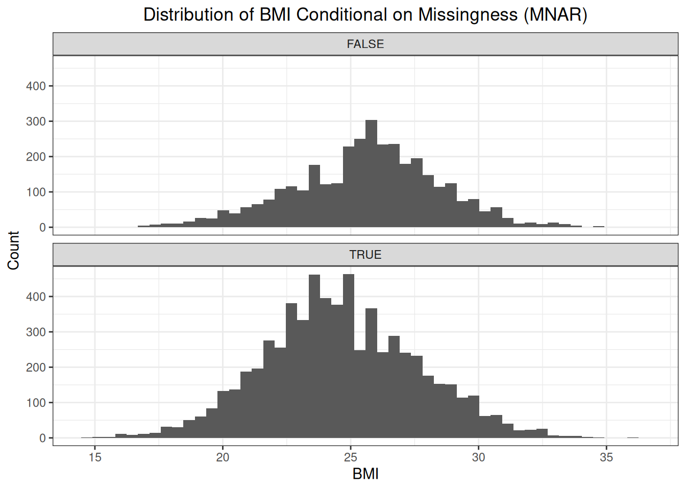
The distribution of the missing BMI values is shifted to the left compared to the distribution of the observed BMI values. This makes sense as the probability of the weight being recorded, and thus the BMI being calculated, is bigger as a patient tends to be overweight or obese.

We know from our simulation that sex does not influence the probability of missigness, nor is there any other factor that influences the probability of missingness, only the outcome itself. Therefore, conditioning on sex, will not eliminate the difference in distribution between observed and missing values.