2 Example Applications
** using the datasets package and information from Wikipedia.
2.1 Abstract
Reynolds (1994) describes a small part of a study of the long-term temperature dynamics of beaver Castor canadensis in north-central Wisconsin. Body temperature was measured by telemetry every 10 minutes for four females, but data from a one period of less than a day for each of two animals is used there
2.2 Introduction:
The beaver (genus Castor) is a large, primarily nocturnal, semiaquatic rodent. Castor includes two extant species, the North American beaver (Castor canadensis) (native to North America) and Eurasian beaver (Castor fiber) (Eurasia). Beavers are known for building dams, canals, and lodges (homes). They are the second-largest rodent in the world (after the capybara). Their colonies create one or more dams to provide still, deep water to protect against predators, and to float food and building material. The North American beaver population was once more than 60 million, but as of 1988 was 6–12 million. This population decline is the result of extensive hunting for fur, for glands used as medicine and perfume, and because the beavers’ harvesting of trees and flooding of waterways may interfere with other land uses.
They are known for their alarm signal: when startled or frightened, a swimming beaver will rapidly dive while forcefully slapping the water with its broad tail, audible over great distances above and below water. This serves as a warning to beavers in the area. Once a beaver has sounded the alarm, nearby beavers will dive and may not reemerge for some time. Beavers are slow on land, but are good swimmers, and can stay under water for as long as 15 minutes.
Beavers are herbivores, and prefer the wood of quaking aspen, cottonwood, willow, alder, birch, maple and cherry trees. They also eat sedges, pondweed, and water lilies. Beavers do not hibernate, but store sticks and logs in a pile in their ponds, eating the underbark. Some of the pile is generally above water and accumulates snow in the winter. This insulation of snow often keeps the water from freezing in and around the food pile, providing a location where beavers can breathe when outside their lodge.
2.3 Methods
We use the followiing procedures to measure the temperature in the beavers:
We capture the beaver
We used a termometer
We measure the temperature
beaver <- datasets::beaver1 # beaver datasets( infromation abouton body temperature measurements at 10 minute intervals.)
beaver2 <- datasets::beaver2

beaver <- rbind(beaver, beaver2) # To make a larger dataset
i <- dim(beaver)[1]/2
beaver$sp <- c(rep( "Castor canadiensis",i), rep( "Castor fiber",i))
beaver$sp <- as.factor(beaver$sp)

summary(beaver)
## day time temp activ
## Min. :307.0 Min. : 0 Min. :36.33 Min. :0.0000
## 1st Qu.:307.0 1st Qu.:1030 1st Qu.:36.85 1st Qu.:0.0000
## Median :346.0 Median :1475 Median :36.99 Median :0.0000
## Mean :327.9 Mean :1375 Mean :37.21 Mean :0.3178
## 3rd Qu.:346.0 3rd Qu.:1920 3rd Qu.:37.64 3rd Qu.:1.0000
## Max. :347.0 Max. :2350 Max. :38.35 Max. :1.0000
## sp
## Castor canadiensis:107
## Castor fiber :107
##
##
##
## What if we are interested to look the full dataset?, but 200 rows is too long to show it, imagine 1000, 2000, 3000 observations ?
DT::datatable(beaver, rownames = F, caption = "Beaver measurements", filter = list(position="top"))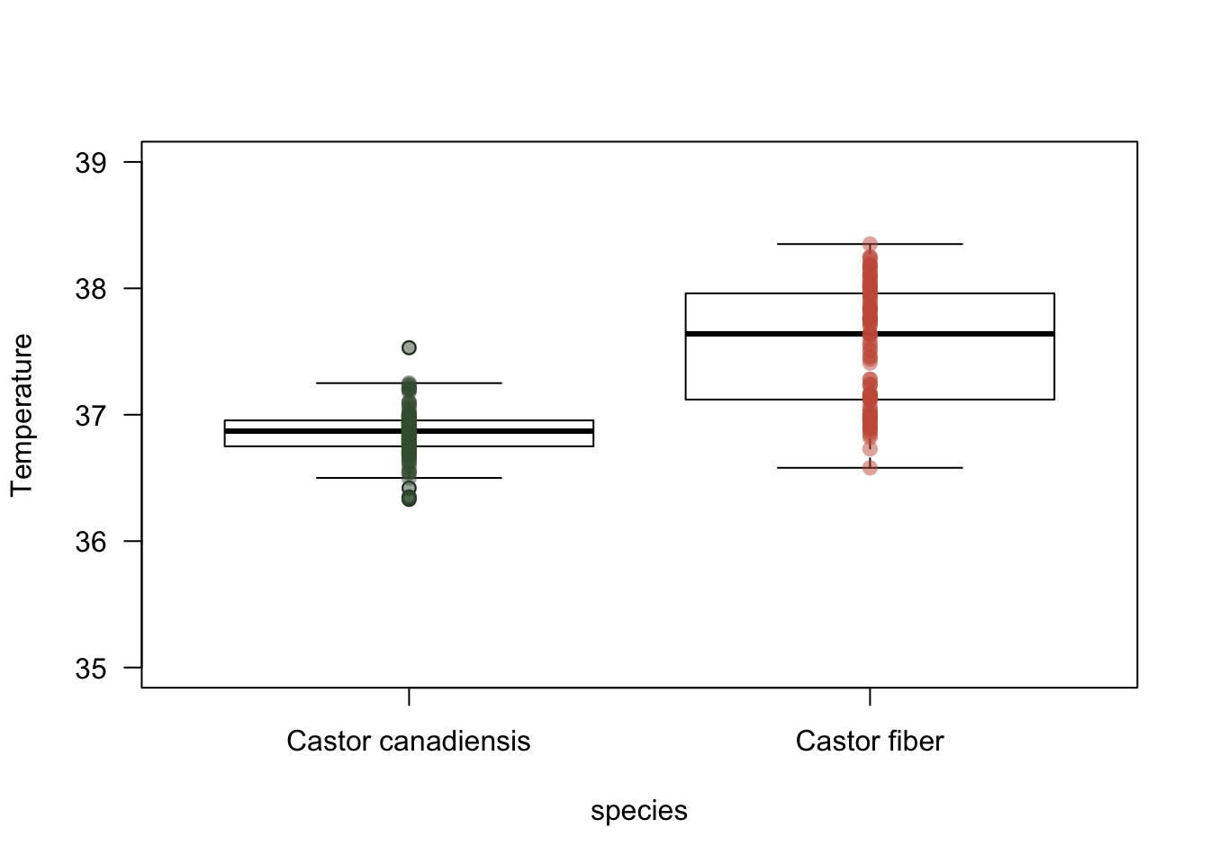
Figure 2.1: Differences of T between tho beaver species
library(pander) #devtools::install_github("Rapporter/pander")
t <- t.test(temp ~ sp, beaver )
pander(t, caption = "T test between beaver data")| Test statistic | df | P value | Alternative hypothesis |
|---|---|---|---|
| -14.24 | 143.1 | 3.218e-29 * * * | two.sided |
| mean in group Castor canadiensis | mean in group Castor fiber |
|---|---|
| 36.86 | 37.55 |
Figure 2.1 shows that beavers from Canada have significant differences in their temperature when compared to bevers from Europe
2.3.1 Body temperature in relation to time
par ( las = 1)
# adding colors to dataset
beaver$col <- c(rep(c.c, i), rep(c.f, i))


plot(temp~time, col = alpha(col, 0.7), pch=16, beaver)
legend("bottomleft",legend = unique(beaver$sp), col = unique(beaver$col),
       pch = 16, bty = "n", cex = 0.7)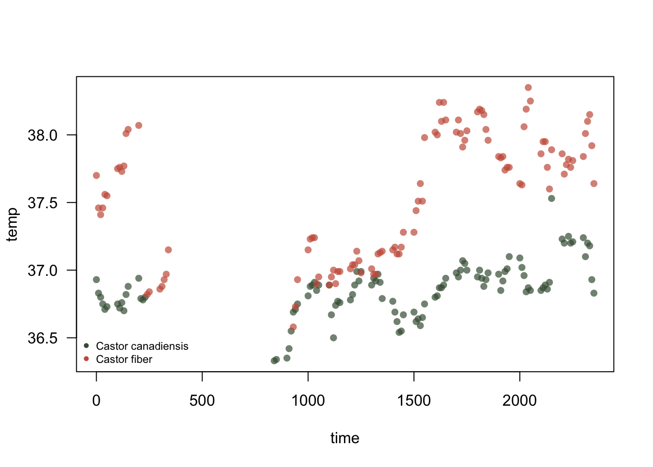
Figure 2.2: Relationship between beaver body temperature and time of day
library(plotly)## Loading required package: ggplot2##
## Attaching package: 'plotly'## The following object is masked from 'package:ggplot2':
##
## last_plot## The following object is masked from 'package:stats':
##
## filter## The following object is masked from 'package:graphics':
##
## layoutplot_ly(beaver, x= ~time,
y = ~temp,
color = ~sp,
colors = ~col,
type = "scatter",
mode = "markers",
text = ~paste("day:",day))c.can <- lm(temp~time, beaver[beaver$sp == "Castor canadiensis",])
c.fib <- lm(temp~time, beaver[beaver$sp == "Castor fiber",])2.4 Final Results
library(memisc)## Loading required package: lattice## Loading required package: MASS##
## Attaching package: 'MASS'## The following object is masked from 'package:plotly':
##
## select##
## Attaching package: 'memisc'## The following objects are masked from 'package:plotly':
##
## rename, style## The following object is masked from 'package:scales':
##
## percent## The following objects are masked from 'package:stats':
##
## contr.sum, contr.treatment, contrasts## The following object is masked from 'package:base':
##
## as.arraymtable <- mtable("C.canadiensis" = c.can, "C.fiber" = c.fib,
summary.stats = c('R-squared','F','p'))plot(temp~time, col = alpha(col, 0.7), pch=16, beaver)
legend("bottomleft",legend = unique(beaver$sp), col = unique(beaver$col),
pch = 16, bty = "n", cex = 0.9)
abline(c.can, lty = 1, lwd = 2, col = c.c)
abline(c.fib, lty = 1, lwd = 2, col = c.f)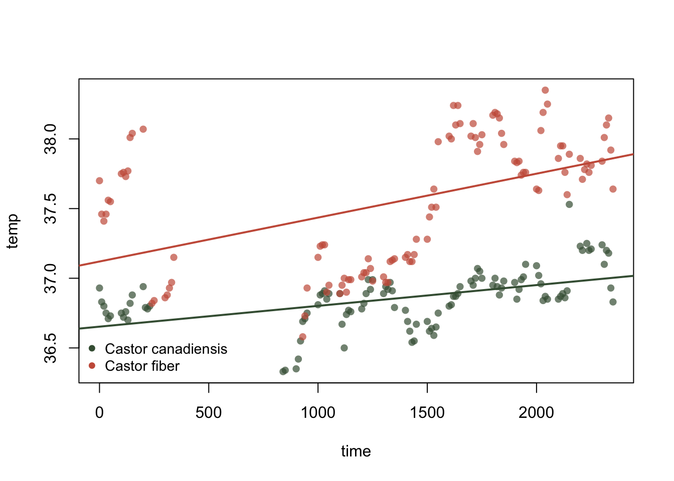
pander(mtable,caption = "linear models for beavers")| C.canadiensis | C.fiber | |
|---|---|---|
| (Intercept) | 36.653*** (0.038) |
37.120*** (0.088) |
| time | 0.000*** (0.000) |
0.000*** (0.000) |
| R-squared | 0.3 | 0.2 |
| F | 36.7 | 30.5 |
| p | 0.0 | 0.0 |
More about pander (http://rapporter.github.io/pander/)
2.5 Where do beavers live?
library(rgbif) # API to GBIF
keys <- sapply(unique(beaver$sp), function(x) name_backbone(name=x)$speciesKey, USE.NAMES=FALSE) # Get unique key id of species
dist <- occ_search(keys, hasCoordinate = TRUE, limit = 200) # Search occurrences
c.can.cor <- dist$`2439838`$data # Castor canadiensis
c.fib.cor <- dist$`4409131`$data # Castor fiber


match <- names(c.fib.cor) %in% names(c.can.cor)
c.fib.cor<-c.fib.cor[,match]

match2 <- names(c.can.cor) %in% names(c.fib.cor)
coor <- rbind(c.can.cor[,match2],c.fib.cor)
coor$col <- ifelse(coor$name == "Castor canadensis", c.c, c.f)names(coor)## [1] "name"
## [2] "key"
## [3] "decimalLatitude"
## [4] "decimalLongitude"
## [5] "issues"
## [6] "datasetKey"
## [7] "publishingOrgKey"
## [8] "publishingCountry"
## [9] "protocol"
## [10] "lastCrawled"
## [11] "lastParsed"
## [12] "crawlId"
## [13] "extensions"
## [14] "basisOfRecord"
## [15] "taxonKey"
## [16] "kingdomKey"
## [17] "phylumKey"
## [18] "classKey"
## [19] "orderKey"
## [20] "familyKey"
## [21] "genusKey"
## [22] "speciesKey"
## [23] "scientificName"
## [24] "kingdom"
## [25] "phylum"
## [26] "order"
## [27] "family"
## [28] "genus"
## [29] "species"
## [30] "genericName"
## [31] "specificEpithet"
## [32] "taxonRank"
## [33] "dateIdentified"
## [34] "year"
## [35] "month"
## [36] "day"
## [37] "eventDate"
## [38] "modified"
## [39] "lastInterpreted"
## [40] "references"
## [41] "license"
## [42] "identifiers"
## [43] "facts"
## [44] "relations"
## [45] "geodeticDatum"
## [46] "class"
## [47] "countryCode"
## [48] "country"
## [49] "rightsHolder"
## [50] "identifier"
## [51] "verbatimEventDate"
## [52] "datasetName"
## [53] "verbatimLocality"
## [54] "gbifID"
## [55] "collectionCode"
## [56] "occurrenceID"
## [57] "taxonID"
## [58] "recordedBy"
## [59] "catalogNumber"
## [60] "http...unknown.org.occurrenceDetails"
## [61] "institutionCode"
## [62] "rights"
## [63] "identificationID"
## [64] "coordinateUncertaintyInMeters"
## [65] "occurrenceRemarks"
## [66] "col"library(leaflet)
leaflet(coor) %>% addTiles() %>%
addCircles(lng = ~decimalLongitude, lat = ~decimalLatitude,radius = 10,
col = ~col,popup = ~dateIdentified)Figure 2.3: Distributions of beavers in the world