Chapter 12 Resampling

Resampling consists in re-using our data several times in smart ways, particularly when one doesn’t want to make too many assumptions about the underlying distribution that is generating our data. There are many reasons for which one would want to re-use one’s data, and today we’ll look at three different cases in which resampling can help us:

Estimating confidence intervals (using bootstrapping)
Testing a model (using permutation)
Evaluating model fit (using cross-validation)

For these exercises, we’ll use the tidyverse library, so let’s load it first.

library("tidyverse")

12.1 The bootstrap

We’ll use a dataset published by Allison and Cicchetti (1976). In this study, the authors studied the relationship between sleep and various ecological and morphological variables across a set of mammalian species: https://science.sciencemag.org/content/194/4266/732

Let’s start by loading the data into a table:

allisontab <- tibble(read.csv("Data_allison.csv"))

This dataset contains several variables related to various body measurements and measures of sleep in different species. Note that some of these are continuous, while others are discrete and ordinal.

summary(allisontab)

##    Species              BodyWt            BrainWt         NonDreaming    
##  Length:62          Min.   :   0.005   Min.   :   0.14   Min.   : 2.100  
##  Class :character   1st Qu.:   0.600   1st Qu.:   4.25   1st Qu.: 6.250  
##  Mode  :character   Median :   3.342   Median :  17.25   Median : 8.350  
##                     Mean   : 198.790   Mean   : 283.13   Mean   : 8.673  
##                     3rd Qu.:  48.202   3rd Qu.: 166.00   3rd Qu.:11.000  
##                     Max.   :6654.000   Max.   :5712.00   Max.   :17.900  
##                                                          NA's   :14      
##     Dreaming       TotalSleep       LifeSpan         Gestation     
##  Min.   :0.000   Min.   : 2.60   Min.   :  2.000   Min.   : 12.00  
##  1st Qu.:0.900   1st Qu.: 8.05   1st Qu.:  6.625   1st Qu.: 35.75  
##  Median :1.800   Median :10.45   Median : 15.100   Median : 79.00  
##  Mean   :1.972   Mean   :10.53   Mean   : 19.878   Mean   :142.35  
##  3rd Qu.:2.550   3rd Qu.:13.20   3rd Qu.: 27.750   3rd Qu.:207.50  
##  Max.   :6.600   Max.   :19.90   Max.   :100.000   Max.   :645.00  
##  NA's   :12      NA's   :4       NA's   :4         NA's   :4       
##    Predation        Exposure         Danger     
##  Min.   :1.000   Min.   :1.000   Min.   :1.000  
##  1st Qu.:2.000   1st Qu.:1.000   1st Qu.:1.000  
##  Median :3.000   Median :2.000   Median :2.000  
##  Mean   :2.871   Mean   :2.419   Mean   :2.613  
##  3rd Qu.:4.000   3rd Qu.:4.000   3rd Qu.:4.000  
##  Max.   :5.000   Max.   :5.000   Max.   :5.000  
##

We’ll start by comparing the body weight (BodyWt) and brain weight (BrainWt) measurements from all the species. As these are measurements that span multiple orders of magnitude, we’lll log-scale them before analyzing them. Later on, we’ll also use the amount of time a species sleeps (TotalSleep) as well, so let’s remove any rows that have missing data for any of these 3 variables.

# Remove rows with missing data in columns of interest 
allisontab <- filter(allisontab,!is.na(BrainWt) & !is.na(BodyWt) & !is.na(TotalSleep))
# Log-scale body and brain weight
allisontab <- mutate(allisontab,logBody=log10(BodyWt), logBrain=log10(BrainWt))

Let’s first look at the relationship between body weight and brain weight (now both in log-scale):

plot(allisontab$logBrain,allisontab$logBody)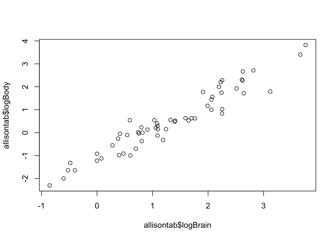

There seems to be a linear relationship here. But how confident are we in this?

We’ll use bootstrapping to assess the strength of this relationship: we’ll build confidence intervals on the slope parameter of a linear regression of logBrain as a function of logBody using as few parametric assumptions as possible. The bootstrap comes to the rescue whenever we don’t want to assume too much about the sampling distribution of our parameter. Below is a function to obtain a single bootstrapped sample from an input dataset. Take a close look at each step.

bootstrap <- function(tab){
  # Preliminary check: if the table is a vector with a single variable, turn it into a matrix
  if(is.null(dim(tab))){tab <- matrix(tab,ncol=1)}
  # Count the number of elements in our data
  numelem <- nrow(tab)
  # Sample indexes with replacement
  bootsidx <- sample(1:numelem, replace=TRUE)
  # Obtain a boostrapped sample by selecting the bootstrapped indexes from the original sample
  final <- tab[bootsidx,]
  # Produce bootstrapped sample as output
  return(final)
}

Let’s see what happens when we run this function on our data.

boots <- bootstrap(allisontab)
plot(boots$logBrain,boots$logBody)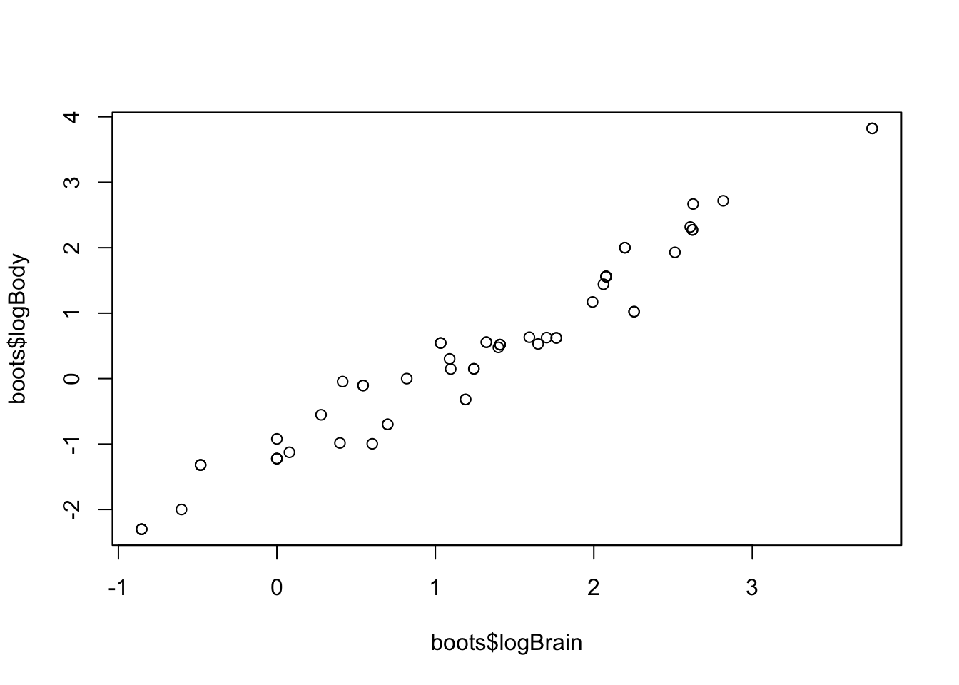

Repeat the above command lines multiple times. What happens?

Let’s estimate a parameter: the slope coefficient in a linear regression of log brain weight on log body weight:

lmmodel <- lm(logBrain ~ logBody, data=allisontab)
estimate <- lmmodel$coeff[2]
estimate

##   logBody 
## 0.7591064

Exercise: try estimating the same parameter from a series of 1000 bootstrapped samples of our original data, and collecting each of the bootstrapped parameters into a vector called “bootsvec”. Hint: you might want to use a for loop or a vectorized sapply() function.

Let’s plot the ecdf of all our estimates, using the function ecdf().

plot(ecdf(bootsvec))
abline(v=estimate,col="red")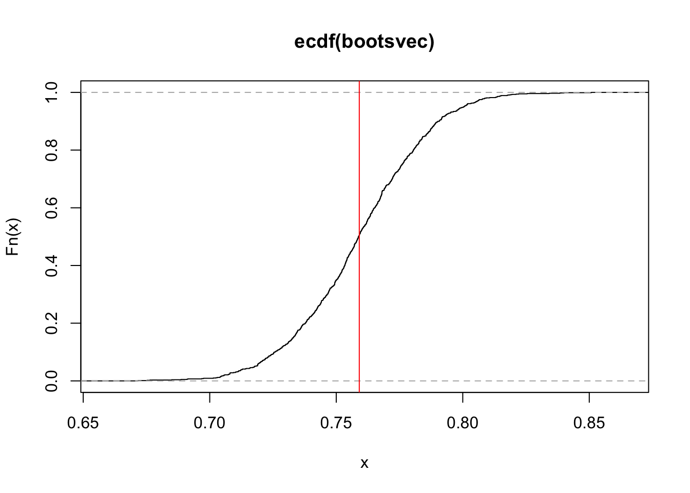

We are now ready to obtain confidence intervals (CIs) of our original parameter estimate, using our bootstrapped distribution. There are multiple ways to obtain CIs from a bootstrapped distribution. Some of these assume that the ECDF has particular properties, while others are more generally applicable:
a) Standard error approach - assumes ECDF is approximately normal
b) Percentile approach - assumes ECDF is symmetric and median-unbiased
c) Pivotal approach - most general, makes almost no assumptions.
These three approaches generally result in very similar CIs, but they differ (slightly) in methodology. In the interest of time, we’ll demonstrate how to run the first two approaches in R. We’ll leave the third approach as an exercise you can do at home (read Box 8-1 in the Edge book for an explanation of it, and a code example).

The standard approach is the most ‘parametric’ of the 3 approaches. Recall from the lecture on properties of estimators that we can obtain CIs from a Normally-distributed summary statistic \(\theta\) by using the standard error of the statistic: \(SE(\hat{\theta}_n)\):

\[(\hat{\theta} - SE(\hat{\theta}_n)q_{97.5\%}, \hat{\theta} + SE(\hat{\theta}_n)q_{97.5\%})\] Where \(q_{97.5\%}\) is a quantile from a standard N(0,1) Normal distribution, and \(SE(\hat{\theta}_n)\) is the standard error (the standard deviation of our estimator). The standard error approach to obtain boostrap confidence intervals proceeds by replacing the standard error \(SE(\hat{\theta}_n)\) with the standard deviation of the bootstrap distribution as a stand-in for it. Let’s call this last value \(SE_b(\hat{\theta}_n)\). Then:

\[(\hat{\theta} - SE_b(\hat{\theta}_n)q_{97.5\%}, \hat{\theta} + SE_b(\hat{\theta}_n)q_{97.5\%})\] In R, we can thus obtain the CI around the mean as follows:

# Let bootsvec be our vector of boostrapped parameters from the previous exercise
bootsmean <- mean(bootsvec)
SEb <- sd(bootsvec)
NormalQ <- qnorm(0.975,mean=0, sd=1)
CIs.bootsSE <- c( bootsmean - SEb*NormalQ, bootsmean + SEb*NormalQ )
names(CIs.bootsSE) <- c("2.5%","97.5%")
CIs.bootsSE

##      2.5%     97.5% 
## 0.7091704 0.8086051

Note that here, we are still using Normal quantiles, which is why this method has a bit of a parametric flavor.

The percentile approach is less ‘parametric’ and simply involves obtaining percentiles of the bootstrap distribution. If we are interested in a 95% CI, for example, we just look for the values of the bootstrap distribution that correspond to the 2.5% percentile and the 97.5% percentile, so that the central bootstrap distribution mass between them adds up to 95%.

Exercise: To obtain the bootstrap-based quantile confidence intervals, compute the 95% quantiles (lower 2.5% and upper 97.5%) of the bootstrap distribution we’ve obtained before.

Compare these confidence intervals to the (highly parametric) CIs that are obtained directly from the linear model, using the function confint, which assumes that the fitted parameter is normally distributed, and does not use any information about bootstraps at all (just the standard error of the fitted model).

CIs.param <- confint(lmmodel)[2,]
CIs.param

##     2.5 %    97.5 % 
## 0.6984844 0.8197284

While it is easy to obtain parametric CIs in this case (as this is a simple linear model), it will be much harder to obtain parametric CIs for more complex models where normality assumptions are harder to justify. Bootstrap-based CIs, in contrast, are obtainable regardless of how complex your model is: you just need to bootstrap your data many times and fit you your model on each bootstraped sample!

12.2 Permutation test

Let’s evaluate the relationship that there is no relationship between logBrain and logBody. Recall that one way to do it would be by using a linear model, and testing whether the value of the fitted slope is significantly different from zero, using a t-test:

summary(lm(logBrain ~ logBody, data=allisontab))

## 
## Call:
## lm(formula = logBrain ~ logBody, data = allisontab)
## 
## Residuals:
##      Min       1Q   Median       3Q      Max 
## -0.75701 -0.21266 -0.03618  0.19059  0.82489 
## 
## Coefficients:
##             Estimate Std. Error t value Pr(>|t|)    
## (Intercept)  0.93507    0.04302   21.73   <2e-16 ***
## logBody      0.75911    0.03026   25.09   <2e-16 ***
## ---
## Signif. codes:  0 '***' 0.001 '**' 0.01 '*' 0.05 '.' 0.1 ' ' 1
## 
## Residual standard error: 0.3071 on 56 degrees of freedom
## Multiple R-squared:  0.9183, Adjusted R-squared:  0.9168 
## F-statistic: 629.2 on 1 and 56 DF,  p-value: < 2.2e-16

This test, however, makes assumptions on our data that sometimes may not be warranted, like large sample sizes and homogeneity of variance. We can perform a more general test that makes less a priori assumptions on our data - a permutation test - as long as we are careful in permuting the appropriate variables for the relationship we are trying to test. In this case, we only have two variables, and we are trying to test whether there is a significant relationship between them. If we randomly shuffle one variable with respect to the other, we should obtain a randomized sample of our data. We can use the following function, which takes in a tibble and a variable of interest, and returns a new tibble in which that particular variable’s values are randomly shuffled.

permute <- function(tab,vartoshuffle){
  # Extract column we wish to shuffle as a vector
  toshuffle <- unlist(tab[,vartoshuffle],use.names=FALSE)
  # The function sample() serves to randomize the order of elements in a vector
  shuffled <- sample(toshuffle)
  # Replace vector in new table (use !! to refer to a dynamic variable name)
  newtab <- mutate(tab, !!vartoshuffle := shuffled )
  return(newtab)
}

Now we can obtain a permuted version of our original data, and compute the slope estimate on this dataset instead:

permuted <- permute(allisontab, "logBrain")
plot(permuted$logBody,permuted$logBrain)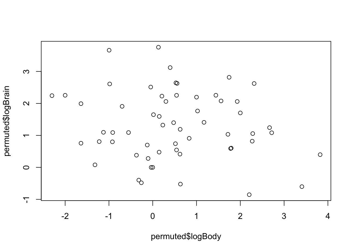

permest <- lm(logBrain ~ logBody, data=permuted)$coeff[2]
permest

##    logBody 
## -0.1099827

Exercise: try estimating the same parameter from a series of 100 permuted versions of our original data, and collecting each of the permuted parameters into a vector called “permvec”.

We now have a distribution of the parameter estimate under the assumption that there is no relationship between these two variables.

Exercise: obtain an empirical one-tailed P-value from this distribution by counting how many of the statistics you obtained from the permuted samples are as large as the one we obtained from our original estimate, and dividing by the total number of permuted samples we have.

12.3 Extra: A ready-made permutation test

The R package coin provides a handy way to apply permutation tests to a wide variety of problems.

if (!require("coin")) install.packages("coin")

## Loading required package: coin

## Loading required package: survival

## 
## Attaching package: 'coin'

## The following object is masked from 'package:infer':
## 
##     chisq_test

## The following object is masked from 'package:scales':
## 
##     pvalue

library("coin") # Library with pre-written permutation tests

The spearman_test() function runs a permutation test of independence between two numeric variables, like the one in the permute() function we just coded above. The advantage is that we don’t need to actually code the function, we can just run the pre-made function in the coin package directly, as long as we know what type of dependency we’re testing. In this case, we perform a test using 1000 permutations (the more permutations, the more exact the test):

spearman_test(TotalSleep ~ log(BodyWt), data=allisontab, distribution=approximate(nresample=1000))

## 
##  Approximative Spearman Correlation Test
## 
## data:  TotalSleep by log(BodyWt)
## Z = -3.8188, p-value < 0.001
## alternative hypothesis: true rho is not equal to 0

Exercise: Perform a permutation test to assess whether there is a significant relationship between log(BrainWt) and TotalSleep. Compare this to the p-value form the t-statistic testing the same relationship in your fitted linear model.

12.4 Extra: A two-category permutation test

Let’s perform a different type of permutation test. In this case, we’ll test whether the mean scores of two categories (for example, the math exam scores from two classrooms) are significantly different from each other.

mathscore <- c(80, 114, 90, 110, 116, 114, 128, 110, 124, 130)
classroom <- factor(c(rep("X",5), rep("Y",5)))
scoretab <- data.frame(classroom, mathscore)

The standard way to test this is using a two-sample t-test, which assumes we have many observations from the two classrooms (do we?) and that these observations come from distributions that have the same variance:

t.test(mathscore~classroom, data=scoretab, var.equal=TRUE)

## 
##  Two Sample t-test
## 
## data:  mathscore by classroom
## t = -2.345, df = 8, p-value = 0.04705
## alternative hypothesis: true difference in means between group X and group Y is not equal to 0
## 95 percent confidence interval:
##  -38.081091  -0.318909
## sample estimates:
## mean in group X mean in group Y 
##           102.0           121.2

Exercise: look at the help menu for the oneway_test in the coin package and find a way to carry out the same type of statistical test as above, but using a permutation procedure. Apply it to the scoretab data defined above. Do you see any difference between the P-values from the t-test and the permutation-based test. Why?

12.5 Permutation recap

To recap then,

If we want to test whether there is a significant relationship (positive or negative) between two variables, we can:
- Run a linear regression (lm()) and obtain the P-value of a t-test checking whether the slope is significantly different from zero (if we have lots of data)
- Or, alternatively, permute one variable with respect to the other many times, using the spearman_test() function (if we are data-limited and don’t want to make too many assumptions on the data).
If we want to test whether two sets of scores are significantly different from each other, we can:
- Use a two-sample t-test t.test() (if we have lots of data)
- Or, alternatively, permute the categories of the scores many times, using the oneway_test() function (if we are data-limited and don’t want to make too many assumptions on the data).

12.6 Validation

We’ll perform a validation exercise to evaluate the error of various models on the data. In this case, we’ll create a predictor for TotalSleep as a function of logBody, using a linear model, and then test how well it does. We’ll first divide our data into a “training” partition - which we’ll use to fit our model - and a separate “test” partition - which we’ll use to test how well our model is doing, and avoid over-fitting. Each partition will be one half of our original data.

# Obtain the number of data points we have
numdat <- dim(allisontab)[1]
# For the training set, randomly sample 50% of the data indexes
trainset <- sample(numdat, round(numdat*0.5))
# For the test set, obtain all indexes that are not in training set
testset <- seq(1,numdat)[-trainset]

Let’s begin by calculating the mean squared error (MSE) between our observations and our predictions in our test partition, after fitting a linear model to our training partition:

# Fit the linear model to the training subset of the data
fit1 <- lm(TotalSleep ~ logBody, data=allisontab,subset=trainset)
# Predict all observations using the fitted linear model
predall <- predict(fit1,allisontab)
# Compute mean squared differences between observations and predictions
sqdiff <- (allisontab$TotalSleep - predall)^2 
# Extract the differences for the test partition
sqdiff.test <- sqdiff[testset]
# Compute the mean squared error
mse1 <- mean(sqdiff.test)

Now, we’ll try to fit our data to 3 more complex models: a quadratic model, a cubic model and a 4-th degree polynomial model, using the function poly:

fit2 <- lm(TotalSleep ~ poly(logBody,2), data=allisontab,subset=trainset)
mse2 <- mean(((allisontab$TotalSleep - predict(fit2,allisontab))^2)[testset])

fit3 <- lm(TotalSleep ~ poly(logBody,3), data=allisontab,subset=trainset)
mse3 <- mean(((allisontab$TotalSleep - predict(fit3,allisontab))^2)[testset])

fit4 <- lm(TotalSleep ~ poly(logBody,4), data=allisontab,subset=trainset)
mse4 <- mean(((allisontab$TotalSleep - predict(fit4,allisontab))^2)[testset])

We can see that the MSE appears to increase for the more complex models. This suggests a simple linear fit performs better at predicting values that were not included in the training set.

Exercise: compute the MSE on the training partition. Compare the resulting values to the MSE on the test partition. What do you observe? Is the difference in errors between the three models as large as when computing the MSE on the test partition? Why do you think this is?

12.7 Cross-validation

We’ll now perform a cross-validation exercise. If you haven’t installed it, you’ll need to install the library boot before loading it. This allows you to perform various resampling techniques, including both bootstrapping and cross-validation.

if(require("boot") == FALSE){install.packages("boot")}

## Loading required package: boot

## 
## Attaching package: 'boot'

## The following object is masked from 'package:survival':
## 
##     aml

library("boot")

The function cv.glm() from the library boot can be used to compute a cross-validation error. This function is designed to work with the glm() function for fitting generalized linear models in R, but we can compute a simple linear regression using glm() as well, and then feed the result into cv.glm():

fit1=glm( TotalSleep ~ logBody, data=allisontab )
# The LOOCV error is computed using the function cv.glm()
cv.err=cv.glm(allisontab,fit1)

The value of the cross-validation error is stored in the first element of the attribute delta of the output of cv.glm. By default, this is a “leave-one-out” cross-validation (LOOCV) error, meaning it computes error by leaving 1 data point out of the fitting and evaluating the error at that data point. The process is iterated over all data points, and the errors are then averaged together. We can obtain the value of the LOOCV error by writing:

cv.err$delta[1]

## [1] 15.97798

Now, let’s compute the LOOCV error for increasingly complex polynomial models (linear, quadratic, cubic, etc.):

CVerr=rep(0,5)
for(m in 1:5){
  fit=glm(TotalSleep ~ poly(logBody,m), data=allisontab)
  CVerr[m]=cv.glm(allisontab,fit)$delta[1]
}

Exercise: Plot the results of this cross-validation exercise. Which model has the lowest LOOCV error?

The LOOCV error is approximately unbiased for the true prediction error, but often has high variance, and can be computationally expensive when our datasets are large. 5-fold and 10-fold cross-validation are recommended as a good compromise between reduced variance and a bit of bias in the estimation of the prediction error. Let’s try increasing the size of the K-fold partition.

Exercise: Take a look at the help function for cv.glm. Which argument would you modify to be able to compute the 10-fold cross-validation error, instead of the LOOCV error. Can you do this for the five models we tested above? Which model has the lowest cross-validation error now?