Data manipulation and visualization
ACTEX Learning - AFDP: R Session
Example 1: Motor Insurance Claims Data
For this example, we will use the French Motor Third-Part Liability datasets: freMTPL2freq and freMTPL2sev. The datasets contain the frequency and severity of claims for a motor insurance portfolio.
The datasets are from the CASdatasets R-package, which provides a collection of datasets for actuarial science used in the book “Computational Actuarial Science with R” by Arthur Charpentier and Rob Kaas. We do not need to install the package as the dcata is already made available in the data folder of this project.
For more information on how to install the CASdatasets package please check the helper00.R file in the project folder.
RDS files are R’s binary file format for storing a single R object. The readRDS() function reads the R object from the file and returns it to the R environment. The saveRDS() function can be used to save an R object to a file in RDS format.
R allows the user to manage different types of data, such as .Rdata, .rda, .rds, .csv, .txt, .xls, .xlsx, among others. The different types of data can be loaded into R using functions like load(), read.csv(), read.table(), read_excel(), and others. Each of these types of files occupies a specific format in memory.
Here we look at the first few rows of each dataset:
head(freMTPLfreq) PolicyID ClaimNb Exposure Power CarAge DriverAge
1 1 0 0.09 g 0 46
2 2 0 0.84 g 0 46
3 3 0 0.52 f 2 38
4 4 0 0.45 f 2 38
5 5 0 0.15 g 0 41
6 6 0 0.75 g 0 41
Brand Gas Region Density
1 Japanese (except Nissan) or Korean Diesel Aquitaine 76
2 Japanese (except Nissan) or Korean Diesel Aquitaine 76
3 Japanese (except Nissan) or Korean Regular Nord-Pas-de-Calais 3003
4 Japanese (except Nissan) or Korean Regular Nord-Pas-de-Calais 3003
5 Japanese (except Nissan) or Korean Diesel Pays-de-la-Loire 60
6 Japanese (except Nissan) or Korean Diesel Pays-de-la-Loire 60head(freMTPLsev) PolicyID ClaimAmount
1 63987 1172
2 310037 1905
3 314463 1150
4 318713 1220
5 309380 55077
6 309380 7593Inspecting Data
The freMTPLfreq dataset contains the risk features and the claim number, while the freMTPLsev dataset contains the claim amount and the corresponding policy ID.
We can use the glimpse() function from the dplyr package to get a quick overview of the datasets.
Rows: 6
Columns: 10
$ PolicyID  <fct> 1, 2, 3, 4, 5, 6
$ ClaimNb   <int> 0, 0, 0, 0, 0, 0
$ Exposure  <dbl> 0.09, 0.84, 0.52, 0.45, 0.15, 0.75
$ Power     <fct> g, g, f, f, g, g
$ CarAge    <int> 0, 0, 2, 2, 0, 0
$ DriverAge <int> 46, 46, 38, 38, 41, 41
$ Brand     <fct> "Japanese (except Nissan) or Korean", "Japanese (except Niss…
$ Gas       <fct> Diesel, Diesel, Regular, Regular, Diesel, Diesel
$ Region    <fct> Aquitaine, Aquitaine, Nord-Pas-de-Calais, Nord-Pas-de-Calais…
$ Density <int> 76, 76, 3003, 3003, 60, 60Rows: 6
Columns: 2
$ PolicyID <int> 63987, 310037, 314463, 318713, 309380, 309380
$ ClaimAmount <int> 1172, 1905, 1150, 1220, 55077, 7593Check if there are any missing values in the datasets using the any() function. The is.na() function checks for missing values in the dataset.
Data Preparation
The two datasets have a common variable, PolicyID, which can be used as a key to merge the datasets to create a single dataset that contains both the frequency and severity of claims.
Something to notice is that PolicyID is stored as a character variable in the freMTPLfreq dataset and as an integer variable in the freMTPLsev dataset. So, in order to proceed with merging the two sets, we need to transform the PolicyID variable in the freMTPLfreq dataset to an integer type.
Mutate and Merge Data
The mutate() function is used to create a new variable, or to make a modification to an existing one, as in this case, to transform PolicyID as an integer type.
freMTPLfreq <- freMTPLfreq %>%
  mutate(PolicyID = as.integer(PolicyID))
We could have done this with base R as well, using the as.integer() function.
freMTPLfreq$PolicyID <- as.integer(freMTPLfreq$PolicyID)The way to use the $ operator is to access a variable in a data frame. The class() function is used to check the class of the modified object.
We can now combine the two datasets using the merge() function from base R which merges two datasets based on a common variable, in this case, the PolicyID variable.
There are other functions that can be used to merge datasets, such as inner_join(), left_join(), right_join(), and full_join() from the dplyr package, depending on the desired output.
[1] 30 11 [1] "PolicyID" "ClaimNb" "Exposure" "Power" "CarAge"
[6] "DriverAge" "Brand" "Gas" "Region" "Density"
[11] "ClaimAmount" PolicyID ClaimNb Exposure Power CarAge
Min. : 33.0 Min. :1.000 Min. :0.0100 g :6 Min. : 0.000
1st Qu.:377.2 1st Qu.:1.000 1st Qu.:0.4775 i :5 1st Qu.: 0.000
Median :497.0 Median :1.000 Median :0.6500 e :4 Median : 0.000
Mean :506.4 Mean :1.267 Mean :0.5507 j :4 Mean : 2.733
3rd Qu.:703.0 3rd Qu.:1.750 3rd Qu.:0.7150 l :4 3rd Qu.: 6.500
Max. :956.0 Max. :2.000 Max. :0.9600 d :3 Max. :10.000
(Other):4
DriverAge Brand Gas
Min. :22.00 Fiat : 0 Diesel : 5
1st Qu.:38.25 Japanese (except Nissan) or Korean:27 Regular:25
Median :50.00 Mercedes, Chrysler or BMW : 0
Mean :47.97 Opel, General Motors or Ford : 1
3rd Qu.:51.00 other : 0
Max. :78.00 Renault, Nissan or Citroen : 2
Volkswagen, Audi, Skoda or Seat : 0
Region Density ClaimAmount
Ile-de-France :21 Min. : 23 Min. : 73.0
Aquitaine : 5 1st Qu.: 1724 1st Qu.: 580.5
Pays-de-la-Loire : 2 Median : 3121 Median :1048.5
Basse-Normandie : 1 Mean : 9288 Mean :1873.4
Nord-Pas-de-Calais: 1 3rd Qu.:16786 3rd Qu.:1446.8
Bretagne : 0 Max. :27000 Max. :9924.0
(Other) : 0 Filter and Summarize Data
We can filter the data to include only claims greater than 1000 and summarize the total claims by year. The group_by() function is used to group the data by a specific variable, and the reframe() function is used to calculate summary statistics for each group.
Grouping and Summarize total claims by DriverAge
claims_summary <- claims_data_raw %>%
  group_by(DriverAge) %>%
  reframe(TotalClaims = sum(ClaimAmount))

claims_summary
# A tibble: 19 × 2
DriverAge TotalClaims
<int> <int>
1 22 3409
2 24 1418
3 27 508
4 28 1344
5 32 936
6 34 1390
7 35 747
8 36 1449
9 45 1274
10 47 1584
11 49 3532
12 50 3909
13 51 13868
14 53 9105
15 61 302
16 68 1107
17 71 6518
18 74 3332
19 78 471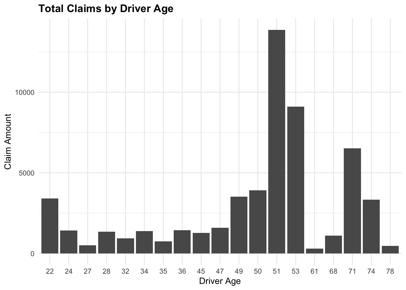
Visualize Projected Claims vs Premium
ggplot(data = claims_data %>% filter(Premium < 10000),
       aes(x = projected_claims, y = Premium)) +
  # Add points
  geom_point() +
  # Add a smooth line
  geom_smooth()+
  labs(title = "Projected Claims vs Premium",
       x = "Projected Claims",
       y = "Premium")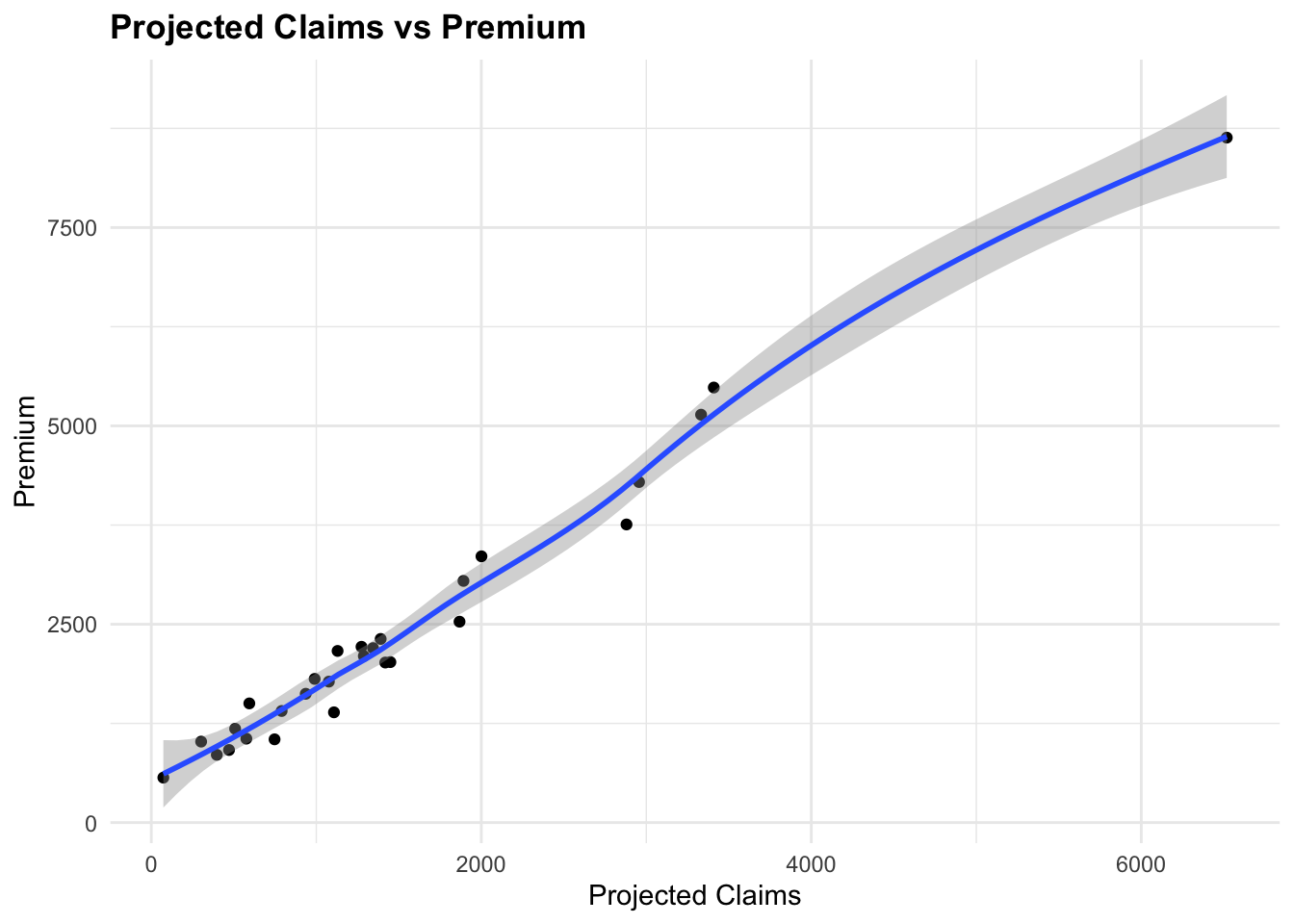
Group Data by Age and Calculate Average Premium
Let’s check the range of the DriverAge variable and group the data by age to calculate the average premium for each age group.
range(claims_data$DriverAge)[1] 22 78Finally, we group the data by 5 years age group and calculate the average premium for each age group using the cut() function to create age groups.
claims_data %>%
  mutate(DriverAge_group = cut_interval(DriverAge,
                                        n = 5)) %>%
  group_by(DriverAge_group) %>%
  reframe(avg_Premium = mean(Premium))
# A tibble: 5 × 2
DriverAge_group avg_Premium
<fct> <dbl>
1 [22,33.2] 2501.
2 (33.2,44.4] 1796.
3 (44.4,55.6] 4439.
4 (55.6,66.8] 1021.
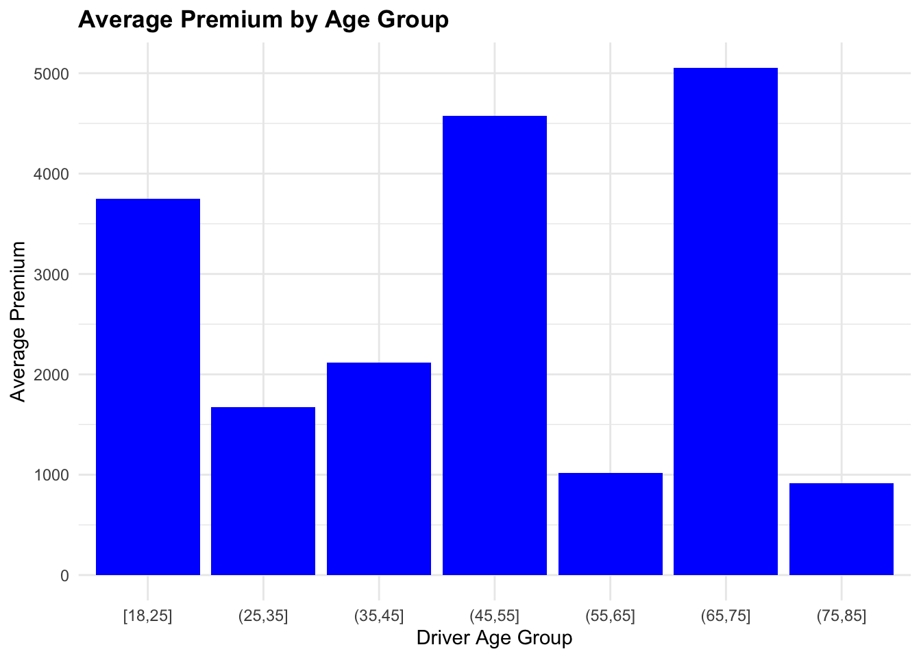
5 (66.8,78] 4020.claims_data_ag <- claims_data %>%
mutate(DriverAge_group = cut(DriverAge,
breaks = c(18, 25, 35,
45, 55, 65,
75, 85, 95, 99),
include.lowest = TRUE)) %>%
arrange(DriverAge_group) %>%
group_by(DriverAge_group) %>%
reframe(avg_Premium = mean(Premium))
claims_data_ag# A tibble: 7 × 2
DriverAge_group avg_Premium
<fct> <dbl>
1 [18,25] 3750.
2 (25,35] 1674.
3 (35,45] 2119.
4 (45,55] 4578.
5 (55,65] 1021.
6 (65,75] 5055.
7 (75,85] 915.