Accessibility

Accessibility map showing travel time to healthcare facilities across Spain

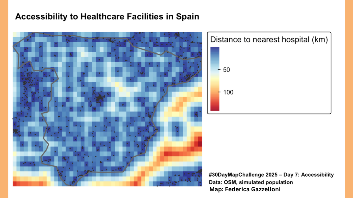
Overview

Accessibility is about how easily people can reach essential services — from hospitals and schools to green spaces and transport.

In this challenge, we visualise travel time to the nearest healthcare facility across Spain, showcasing how geography shapes health opportunities. The map combines population data with spatial travel-time models, illustrating areas with limited access and identifying urban-rural disparities.

Method

Data come from the Global Human Settlement (GHS) and WorldPop datasets, integrated with OpenStreetMap road networks.

Travel time is calculated using a raster-based cost-distance algorithm:

1. Define origin points: centroids of populated grid cells.
   
2. Assign friction surface: speed based on road type and terrain.
3. Compute least-cost path to the nearest healthcare facility.
   
4. Aggregate and visualise results by country or region.

Interpretation

The resulting accessibility map shows striking contrasts:

• Urban cores exhibit the shortest travel times (often under 15 minutes).
• Peripheral and mountain areas may require over an hour to reach care.
• These inequalities persist even in countries with universal healthcare systems.

Such spatial disparities are crucial to understanding health equity, informing decisions on infrastructure investment and service allocation.

# Day 7: Accessibility — #30DayMapChallenge 2025
# Author: Federica Gazzelloni
# Data: OSM hospitals + worldpop population + simplified travel time model

# Load libraries
library(sf)
library(tmap)
library(terra)
library(osmdata)
library(eurostat)
library(dplyr)
library(rnaturalearth)
library(rnaturalearthdata)

# 1. Get country boundaries (Europe)
europe <- ne_countries(continent = "Europe", returnclass = "sf")

# 2. Select a country
spain <- europe %>% filter(admin %in% c("Spain"))

# 3. Download hospitals from OpenStreetMap
spain %>%
  st_bbox() %>%
  st_as_sfc() %>%
  st_transform(crs = 4326) -> spain_bbox

q <- opq(bbox = spain_bbox) %>%
  add_osm_feature(key = "amenity", value = "hospital")

options(timeout = 6000)
hospitals <- osmdata_sf(q)$osm_points %>%
  st_transform(crs = st_crs(spain))
# saveRDS(hospitals, "data/hospitals_spain.rds")

# 4. Create a population raster (using WorldPop or synthetic grid)
# For demonstration, we’ll create a grid and simulate population
r <- rast(spain, res = 0.25) # coarse grid (~25km)
values(r) <- runif(ncell(r), min = 0, max = 1000)
r <- mask(r, vect(spain))

# 5. Compute distance (proxy for travel time)
# Euclidean distance in km as a simplified accessibility measure
hospitals_vect <- vect(hospitals)
dist_rast <- distance(r, y = hospitals_vect) / 1000  # convert m to km

tmap_mode("plot")

map_access <- tm_shape(dist_rast) +
  tm_raster(palette = "rd_yl_bu",
    title="Distance to nearest hospital (km)",
    style = "cont") +
  tm_shape(spain) +
  tm_borders(col = "grey40",lwd = 2) +
  tm_shape(hospitals) +
  # ggpubr::show_point_shapes()
  tm_dots(size = 0.05, 
          shape = 10, 
          col = "grey20") +
  tm_title("Accessibility to Healthcare Facilities in Spain",
           fontface="bold") +
    tm_layout(
      legend.outside = TRUE,
    frame = FALSE,
    main.title.size = 1.2
  ) +
  tm_credits(
    "#30DayMapChallenge 2025 – Day 7: Accessibility\nData: OSM, simulated population",
    size = 0.6, 
    position =  tm_pos_out(pos.h = 0, pos.v = 0.1),
    fontface = "bold")

Save the map

tmap_save(
  tm = map_access,
  filename = "day7_accessibility.png",
  width = 2000,      # pixels (approx. 20 cm at 100 dpi)
  height = 1500,     # adjust as needed
  dpi = 300           # print quality
)

# Optional: also view interactively
# tmap_mode("view")
# map_access