Earth – Unlocking the Power of Data Visualization with R

Mapping Suicide Mortality Across the Planet, Age-standardized death rates due to suicide, 1990-2021

Overview

For this challenge we use data from IHME about suicide death rates per 100,000 people in 2021. We will map the data on a globe projection centered on Europe.

library(tidyverse)
library(sf)
library(rnaturalearth)
library(rnaturalearthdata)

Base Map

Load the data

# world data
world <- ne_countries(scale = "medium", returnclass = "sf")

Set a projection

ortho <- "+proj=ortho +lat_0=30 +lon_0=10"

Add the Oceans

ocean <- st_point(x = c(0,0)) %>%
  st_buffer(dist = 6371000) %>% #6,371km ratios of the earth
  st_sfc(crs = ortho)

# plot Earth as a globe centered on Europe
ggplot(data = world) +
  geom_sf(data = ocean,
          linewidth=1,
          fill = "#92c0e2", 
          color = NA)+
  geom_sf(data = ocean, fill = "#A6CEE3", color = NA) +
  geom_sf(fill = "brown", color = NA, linewidth = 0.2) +
  coord_sf(crs = ortho) +
  theme_void() +
  theme(
    plot.title = element_text(size = 16, face = "bold", hjust = 0.5),
    plot.subtitle = element_text(size = 12, hjust = 0.5)) +
  labs(title = "Earth as Seen from Europe",
       subtitle = "Orthographic projection of the planet")

Load data on Suicides

# read data
suicide_raw <- read.csv("data/IHME_GBD_2021_SUICIDE_1990_2021_TAB_2_ASMR_PERCENT_CHANGE_Y2025M02D12.csv")

This data are collected around the Globe at Region level. We filter only what we need.

suicide <- suicide_raw %>%
  filter(!location_name=="Global",
         measure_name=="Deaths",
         sex_name=="Both",
         age_group_name=="Age-standardized",
         metric_name=="Rate")%>%
  select(location_name,year_id,val)%>%
  group_by(location_name)%>%
  reframe(deaths=sum(val))

suicide %>%  head()

We using IHME GBD super-regions (e.g. Andean Latin America, Western Europe, East Asia, etc.) rather than individual countries. These names don’t exist as geometries in standard shapefiles like rnaturalearth, because they are groupings of countries, not administrative units. To plot them, we’ll need to build regional geometries by merging countries that belong to each IHME region.

library(tibble)

ihme_regions <- tribble(
  ~ihme_region, ~countries,

  # Latin America & Caribbean
  "Andean Latin America", c("Bolivia", "Ecuador", "Peru"),
  "Central Latin America", c("Mexico", "El Salvador", "Guatemala", "Honduras", "Nicaragua", "Costa Rica", "Panama", "Colombia", "Venezuela"),
  "Southern Latin America", c("Argentina", "Chile", "Uruguay"),
  "Tropical Latin America", c("Brazil", "Paraguay"),
  "Caribbean", c("Cuba", "Dominican Republic", "Haiti", "Jamaica", "Trinidad and Tobago", "Puerto Rico", "Bahamas", "Barbados"),

  # Sub-Saharan Africa
  "Western Sub-Saharan Africa", c("Nigeria", "Ghana", "Côte d’Ivoire", "Senegal", "Sierra Leone", "Liberia", "Gambia"),
  "Central Sub-Saharan Africa", c("Cameroon", "Congo", "Gabon", "Equatorial Guinea", "Central African Republic"),
  "Eastern Sub-Saharan Africa", c("Ethiopia", "Kenya", "Uganda", "Tanzania", "Madagascar", "Mozambique", "Malawi"),
  "Southern Sub-Saharan Africa", c("South Africa", "Botswana", "Namibia", "Eswatini", "Lesotho", "Zimbabwe", "Zambia"),

  # Europe
  "Western Europe", c("Austria", "Belgium", "France", "Germany", "Italy", "Luxembourg", "Netherlands", "Portugal", "Spain", "Switzerland", "United Kingdom", "Ireland"),
  "Central Europe", c("Poland", "Czechia", "Slovakia", "Hungary", "Slovenia", "Croatia", "Bosnia and Herzegovina", "Serbia", "Montenegro", "North Macedonia"),
  "Eastern Europe", c("Belarus", "Moldova", "Russia", "Ukraine"),

  # Asia & Pacific
  "East Asia", c("China", "Mongolia", "North Korea", "South Korea"),
  "Southeast Asia", c("Indonesia", "Thailand", "Vietnam", "Malaysia", "Philippines", "Cambodia", "Laos", "Myanmar", "Timor-Leste"),
  "South Asia", c("India", "Pakistan", "Bangladesh", "Nepal", "Bhutan", "Maldives"),
  "Central Asia", c("Kazakhstan", "Uzbekistan", "Kyrgyzstan", "Tajikistan", "Turkmenistan"),
  "Australasia", c("Australia", "New Zealand"),

  # High-income & Other
  "High-income North America", c("United States of America", "Canada"),
  "High-income Asia Pacific", c("Japan", "Singapore", "Brunei Darussalam"),
  "Oceania", c("Papua New Guinea", "Fiji", "Solomon Islands", "Vanuatu"),
  "North Africa and Middle East", c("Algeria", "Egypt", "Libya", "Morocco", "Tunisia", "Saudi Arabia", "Iran", "Iraq", "Israel", "Jordan", "Lebanon", "Syria", "Turkey", "Yemen", "United Arab Emirates", "Qatar", "Oman", "Bahrain", "Kuwait")
)

We use some sf steps:

    st_union() %>%
    st_combine() %>%
    st_make_valid()

region_sf <- ihme_regions %>%
  mutate(
    geometry = purrr::map(countries, ~ {
      geom <- world %>%
        filter(name_long %in% .x) %>%
        st_union() %>%
        st_combine() %>%
        st_make_valid()
      geom[[1]]
    })
  ) %>%
  mutate(geometry = st_sfc(geometry, crs = st_crs(world))) %>%
  st_as_sf()

Then, finally join the region_sf with the suicide data:

earth_data <- region_sf %>%
  left_join(suicide, by = c("ihme_region" = "location_name"))

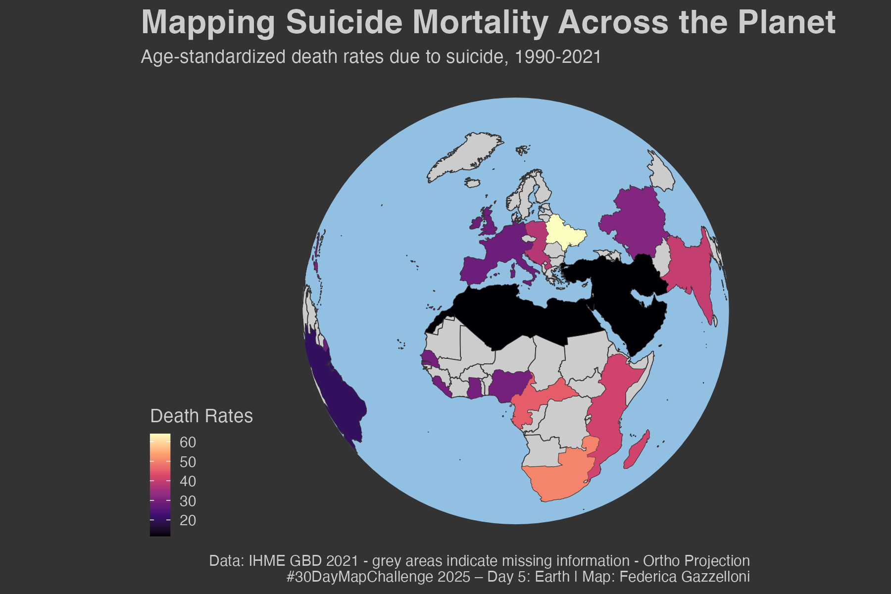
Finally, we can plot the map:

ggplot(earth_data) +
  geom_sf(data = ocean,
          linewidth=1,
          fill = "#92c0e2", 
          color = NA)+
  geom_sf(data = world,
          fill = "grey80", color = "grey20", linewidth = 0.2) +
  geom_sf(aes(fill = deaths), color = "grey20", size = 0.05) +
  coord_sf(crs = ortho) +
  scale_fill_viridis_c(option = "A", 
                       name = "Death Rates") +
  labs(
    title = "Mapping Suicide Mortality Across the Planet",
    subtitle = "Age-standardized death rates due to suicide, 1990-2021",
    caption = "Data: IHME GBD 2021 - grey areas indicate missing information - Ortho Projection\n#30DayMapChallenge 2025 – Day 5: Earth | Map: Federica Gazzelloni"
  )+
  ggthemes::theme_map()+
  theme(text = element_text(color="grey80"),
        legend.key.size = unit(10,"pt"),
        legend.position = "left",
        legend.background = element_rect(fill = NA,colour = NA),
        plot.title.position = "plot",
        plot.title = element_text(size=16,face="bold"))

ggsave("day5_earth.png", 
       width = 6, height = 4, 
       bg="grey20")