Polygons

Global polygon data for mapping disease burden (DALYs) worldwide - Robison Projection

Overview

Data for this challenge comes from the hmsidwR package, which includes global polygon data for mapping disease burden (DALYs) worldwide.

Load Libraries and Data

library(tidyverse)
library(hmsidwR)
library(sf)

data(idDALY_map_data)

To gain more info about the data:

?idDALY_map_data

plot(idDALY_map_data)

Working with Global Projections and Polygons

To plot the map’s polygons to work properly in a different global projection such as the Robinson projection, some preprocessing is needed.

When I first plotted the global polygons under Robinson projection, I noticed strange lines crossing Russia and the equator. These were caused by polygons that were invalid or crossed the ±180° meridian, a common issue in global datasets where countries span the dateline.

To fix this, I followed a few steps:

1. Make sure the geometries are right with st_make_valid(), this removes self-intersections and other inconsistencies.

# 1. Make valid (repairs self-intersections)
idDALY_clean <- st_make_valid(idDALY_map_data)

2. Split multipolygons into individual polygon parts using st_cast(), ensuring that each island or country segment was treated separately.

# 2. Break apart multipolygons into individual polygon pieces
idDALY_clean <- idDALY_clean |>
  st_cast("MULTIPOLYGON") |>
  st_cast("POLYGON", warn = FALSE)

3. Wrapped polygons at the dateline with st_wrap_dateline(), so that shapes crossing the ±180° longitude were properly split and would not draw straight lines across the map.

# 3. Split polygons that cross the dateline
idDALY_clean <- st_wrap_dateline(idDALY_clean, options = c("WRAPDATELINE=YES", "DATELINEOFFSET=180"))

4. Reprojected to Robinson with st_transform(), so the data could be displayed correctly on a flat, visually pleasing projection.

# 4. Reproject to Robinson
idDALY_robin <- st_transform(idDALY_clean, "+proj=robin")

5. Assigned unique polygon IDs to maintain proper grouping in ggplot2.

# 5. Assign a unique polygon id for grouping
idDALY_robin <- idDALY_robin |>
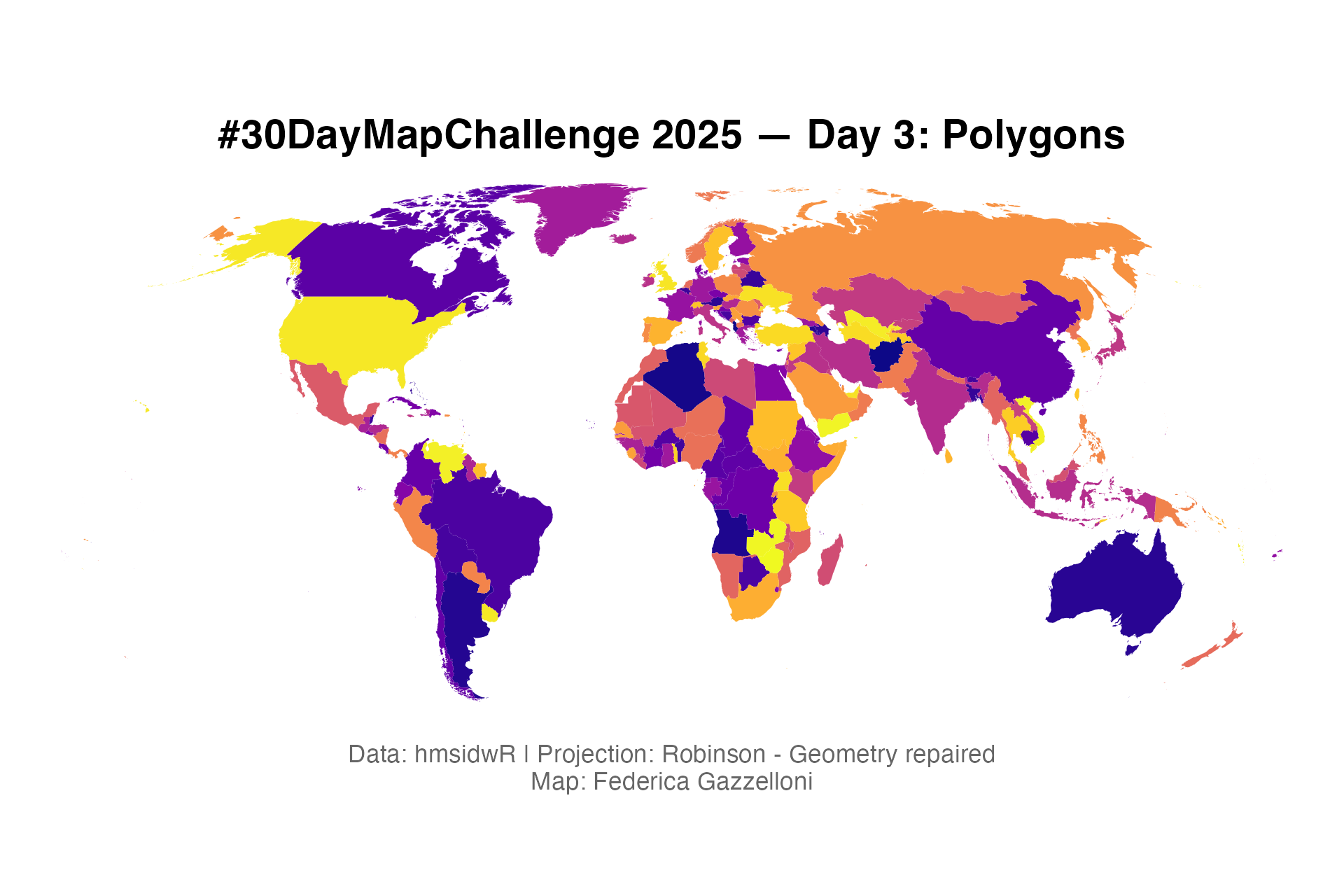
  mutate(poly_id = row_number())

These steps removed the unwanted lines and allowed the polygons to render smoothly in any projection, giving a clean, accurate global map for the Day 3 challenge.

Finally, I plotted the cleaned and reprojected polygons:

# 6. Plot
ggplot(idDALY_robin) +
  geom_sf(aes(fill = location_name, 
              group = poly_id), 
          show.legend = FALSE,
          color = NA) +
  coord_sf(crs = st_crs(idDALY_robin)) +
  theme_void() +
  scale_fill_viridis_d(option = "C") +
  labs(title = "#30DayMapChallenge 2025 — Day 3: Polygons",
       caption = "Data: hmsidwR | Projection: Robinson - Geometry repaired\nMap: Federica Gazzelloni") +
  theme(plot.title = element_text(face = "bold", hjust = 0.5),
        plot.caption = element_text(size = 8, 
                                colour = "grey40", hjust = 0.5))

ggsave("day3_polygons.png", height = 4, width = 6, dpi = 320)

Explanation of the Issue with Polygons and Global Projections

Most global shapefiles (like those used in {hmsidwR}) are stored in longitude/latitude (EPSG:4326), so the world is represented as coordinates ranging from -180° to +180°.

But here’s the catch:

• Countries like Russia, USA (Alaska), and Fiji span across the antimeridian (the ±180° meridian).
• In raw coordinate form, these countries can have polygons whose edges go from +179° → -179°, which looks fine on a globe but breaks on a flat map.
• When you reproject such data (for example, to the Robinson projection), the reprojection algorithm doesn’t wrap those edges, it literally draws a straight line between +179° and -179°, which slices across the map (through the Pacific, or even across the equator).