library(elevatr)
library(terra)
library(sf)
library(ggplot2)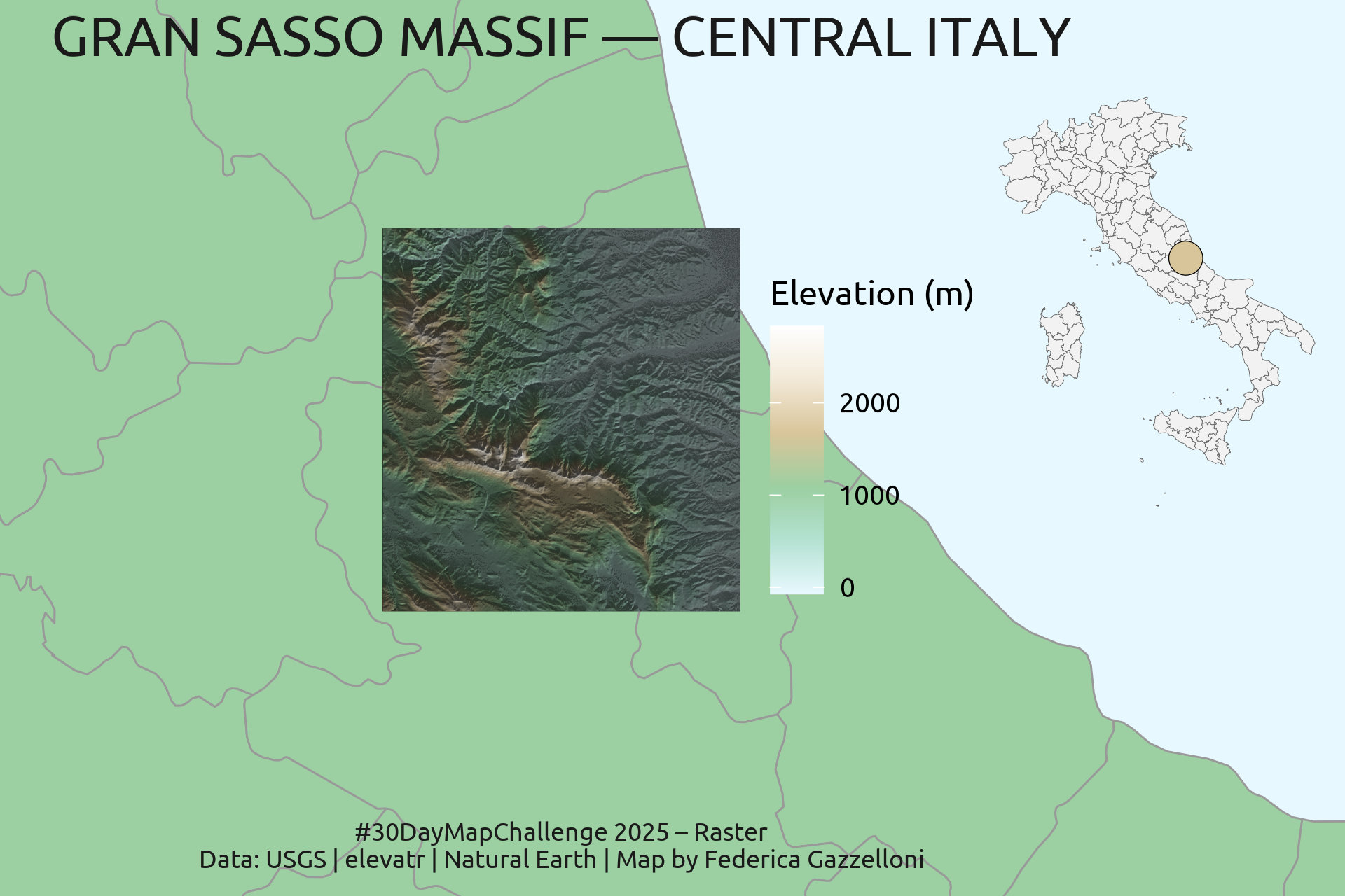 ## Overview
The Gran Sasso Massif is a prominent mountain range located in central Italy, known for its stunning landscapes and significant geological features. This raster map visualizes the elevation of the Gran Sasso Massif and its surrounding areas using high-resolution elevation data. The map employs various shading techniques to enhance the three-dimensional appearance of the terrain, providing a detailed view of the mountainous region.
library(rnaturalearth)
library(rnaturalearthdata)

# Download admin level-1 boundaries
admin1 <- ne_states(country = "Italy", returnclass = "sf")

# Filter a broader area around Abruzzo
region_bg <- admin1[
  admin1$region %in% c("Abruzzo", "Lazio", "Marche", "Umbria", "Molise", "Toscana"),
]ggplot() +
geom_sf(data = admin1) +
geom_sf(data = region_bg,
fill = "lightblue", color = "darkblue", size = 0.5) +
theme_minimal()# -----------------------------
# Font Setup (Elegant Title)
# -----------------------------
library(showtext)
library(sysfonts)
font_add_google("Ubuntu", "ubuntu")
showtext_auto()
showtext_opts(dpi = 320)# -----------------------------
# 1) Bounding box
# -----------------------------
# ~30 km around Gran Sasso
bbox <- st_as_sf(st_as_sfc(st_bbox(c(
xmin = 13.30,
xmax = 14.00,
ymin = 42.25,
ymax = 42.80
), crs = 4326)))# -----------------------------
# 2) High-resolution elevation
# -----------------------------
dem <- get_elev_raster(
locations = bbox,
z = 10, # resolution
clip = "bbox"
)
dem_t <- rast(dem)# -----------------------------
# 3) Shading Layers
# -----------------------------
# Terrain derivatives
slope <- terrain(dem_t, "slope", unit = "radians")
aspect <- terrain(dem_t, "aspect", unit = "radians")
# Hillshade - multi-directional effect for “3D” look
hs1 <- shade(slope, aspect, angle = 40, direction = 315)
hs2 <- shade(slope, aspect, angle = 60, direction = 45)
hillshade <- (hs1 * 0.6 + hs2 * 0.4)
# Curvature shading (adds fine texture)
curve <- terrain(dem_t, "flowdir")
curve <- (curve - min(curve[], na.rm=TRUE)) /
(max(curve[], na.rm=TRUE) - min(curve[], na.rm=TRUE))# -----------------------------
# 4) Convert to df for ggplot
# -----------------------------
df_dem <- as.data.frame(dem_t, xy = TRUE, na.rm = TRUE)
names(df_dem)[3] <- "elevation"
df_hs <- as.data.frame(hillshade, xy = TRUE, na.rm = TRUE)
names(df_hs)[3] <- "hs"
df_curve <- as.data.frame(curve, xy = TRUE, na.rm = TRUE)
names(df_curve)[3] <- "curve"
# Merge rasters
df <- Reduce(function(a, b) merge(a, b, by = c("x", "y"), all = TRUE),
list(df_dem, df_hs, df_curve))
# saveRDS(df, "data/day29_raster_df.rds")# -----------------------------
# 5) Astonishing Map
# -----------------------------
ggplot(df) +
geom_raster(aes(x, y, fill = elevation)) +
geom_raster(aes(x, y, alpha = hs * 1.2)) +
geom_raster(aes(x, y, alpha = curve * 0.3)) +
# Gold elevation palette
scale_fill_gradientn(
colours = c("#e8f8ff", # pale blue (low)
"#b4e2d2", # mint
"#9ccfa1", # soft green
"#d8c59a", # sand
"#f2e9d8", # warm light
"#ffffff"), # snow
name = "Elevation (m)"
) +
scale_alpha(range = c(0, 0.7), guide = "none") +
coord_equal() +
theme_void(base_family = "ubuntu") +
theme(plot.title = element_text(size = 20, color = "white",
hjust = 0.95, vjust = 1),
plot.caption = element_text(size = 8, color = "grey70",
hjust = 0.95, vjust = -1),
legend.position = "none") +
labs(title = "GRAN SASSO MASSIF — CENTRAL ITALY",
caption = "#30DayMapChallenge 2025 – Raster\nData: USGS | elevatr | Map by Federica Gazzelloni"
)ggsave("day29_raster.png", width = 8, height = 6, dpi = 320)base_map <- ggplot() +
# ------------------------------------------
# BASE MAP (POLYGONS) — placed first
# ------------------------------------------
geom_sf(
data = admin1,
fill = "#9ccfa1",
color = "grey60",
linewidth = 0.3,
) +
# ------------------------------------------
# RASTER LAYERS (on top)
# ------------------------------------------
geom_raster(data = df, aes(x, y, fill = elevation)) +
geom_raster(data = df, aes(x, y, alpha = hs * 1.2)) +
geom_raster(data = df, aes(x, y, alpha = curve * 0.3)) +
# Palettes
scale_fill_gradientn(
colours = c("#e8f8ff","#b4e2d2","#9ccfa1",
"#d8c59a","#f2e9d8","#ffffff"),
name = "Elevation (m)"
) +
scale_alpha(range = c(0, 0.75), guide = "none") +
# ------------------------------------------
# COORDINATE SYSTEM
# ------------------------------------------
coord_sf(
xlim = c(13.3, 14),
ylim = c(42, 43),
expand = TRUE,
clip = "off")
base_map# ------------------------------------------
# 5) THEME
# ------------------------------------------
main_map <- base_map +
labs(title = "GRAN SASSO MASSIF — CENTRAL ITALY",
caption = "#30DayMapChallenge 2025 – Raster\nData: USGS | elevatr | Natural Earth | Map by Federica Gazzelloni\n")+
theme_void(base_family = "ubuntu") +
theme(plot.title = element_text(size = 18,
color = "grey10",hjust = 0.5),
plot.caption = element_text(size = 8, color = "grey10",
hjust = 0.5),
legend.background = element_blank())
main_mapAdd an insect map
library(rnaturalearth)
library(rnaturalearthdata)
library(ggplot2)
library(sf)

# -----------------------------
# Gran Sasso centroid to plot on inset
# -----------------------------
gran_sasso_pt <- st_centroid(bbox)  # use your main bbox centroid
inset_map <- ggplot() +
geom_sf(data = admin1, fill = "grey95", color = "grey40", linewidth = 0.1) +
geom_sf(data = gran_sasso_pt,
color = "black", size = 5, shape = 21, stroke=0.2,
fill = "#d8c59a") +
theme_void() +
theme(plot.background = element_rect(fill=NA, color=NA))
inset_maplibrary(cowplot)
inset_grob <- ggdraw(inset_map)
inset_grobbbox
# xlim = c(13.3, 14),
# ylim = c(42, 43),main_map +
annotation_custom(
ggplotGrob(inset_map),
xmin = 14.5, xmax = 15.2, # adjust position
ymin = 42.2, ymax = 43.2
)ggsave("day29_raster.png",
width = 6, height = 4,
bg = "#e8f8ff",
dpi = 320)