Black

Etna volcano elevation contours on a black background

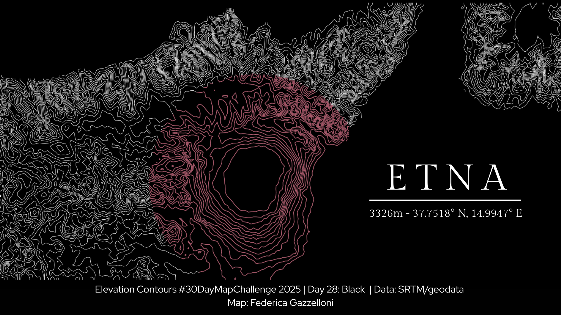
Overview

This Black Themed Map is built using R and various geospatial libraries. The map showcases the Etna volcano area with elevation contours on a black background.

library(terra)
library(ggplot2)
library(sf)

Font Setup

library(showtext)
library(sysfonts)
font_add_google(name = "Ubuntu", family = "Ubuntu")
showtext_auto()
showtext_opts(dpi = 300)

# 1) Download an elevation raster around Mt. Etna
# Using geodata::elevation_30s gives a global DEM; we crop to Etna
library(geodata)
dem <- elevation_30s(country = "ITA", path = tempdir())

# Etna bounding box
etna <- ext(14, 16, 37.5, 38.2)
dem_etna <- crop(dem, etna)

# Convert to stars for ggplot
library(stars)
dem_st <- st_as_stars(dem_etna)

ggplot() +
  geom_stars(data = dem_st) +
  scale_fill_viridis_c()

# 2) Build contours
contours <- st_as_sf(st_contour(dem_st, contour_lines = 200))

# 3) Plot in pure black theme
plot1 <- ggplot() +
  geom_sf(data = contours, 
          color = "grey90", size = 0.2, alpha = 0.6) +
  coord_sf(expand = T,clip = "off") +
  labs(title = "Etna",
       subtitle("3326m - 37.7518° N, 14.9947° E"),
       caption = "Elevation Contours\n#30DayMapChallenge 2025 | Day 28: Black\nData: SRTM / geodata | Map: Federica Gazzelloni") +
  theme_void() +
  theme(text = element_text(color = "grey90", family= "Ubuntu"),
        plot.title= element_blank(),
        plot.caption = element_blank(),
        plot.background = element_rect(fill = "black", color = "black"),
        panel.background = element_rect(fill = "black", color = "black")
  ) 
plot1

Focus on a Point of Interest (POI) with a buffer/circle

Create a circle of a given radius around a POI (point of interest) to crop/filter the original OSM data “down to size”. source: https://thetidytrekker.com/post/making-circular-maps/making-circular-maps.html

crs_data <- unname(st_crs(contours$geometry)$wkt) 
feature_names <- names(contours)

POI = c(
  lat =37.74864,
  long = 15.00461
)
POI

dist <-  30000
#Circle "data" used to crop/filter the original OSM data "down to size"--------
circle <- enframe(POI) |>
  pivot_wider() |>
  st_as_sf(coords = c("long", "lat"), crs = crs_data) |>
  st_buffer(dist = dist) |>
  st_transform(crs = crs_data)

ggplot(circle)+
  geom_sf(fill=NA,color="red")

contours_circle <- st_intersection(circle,contours)

ggplot()+
  geom_sf(data = contours,linewidth=0.1,color="white")+
  geom_sf(data = contours_circle,linewidth=0.2,color="#a85769")+
  coord_sf(expand=T,clip="off") +
  theme_void()+
  theme(
    plot.background = element_rect(fill = "black", color = "black"),
    panel.background = element_rect(fill = "black", color = "black")
  )

# save final plot
ggsave("day28_black2.png",
       bg = "black",
       width = 6,
       height = 4,
       dpi = 320)