library(sf)
library(rnaturalearth)
library(dplyr)
library(ggplot2)
library(stringr)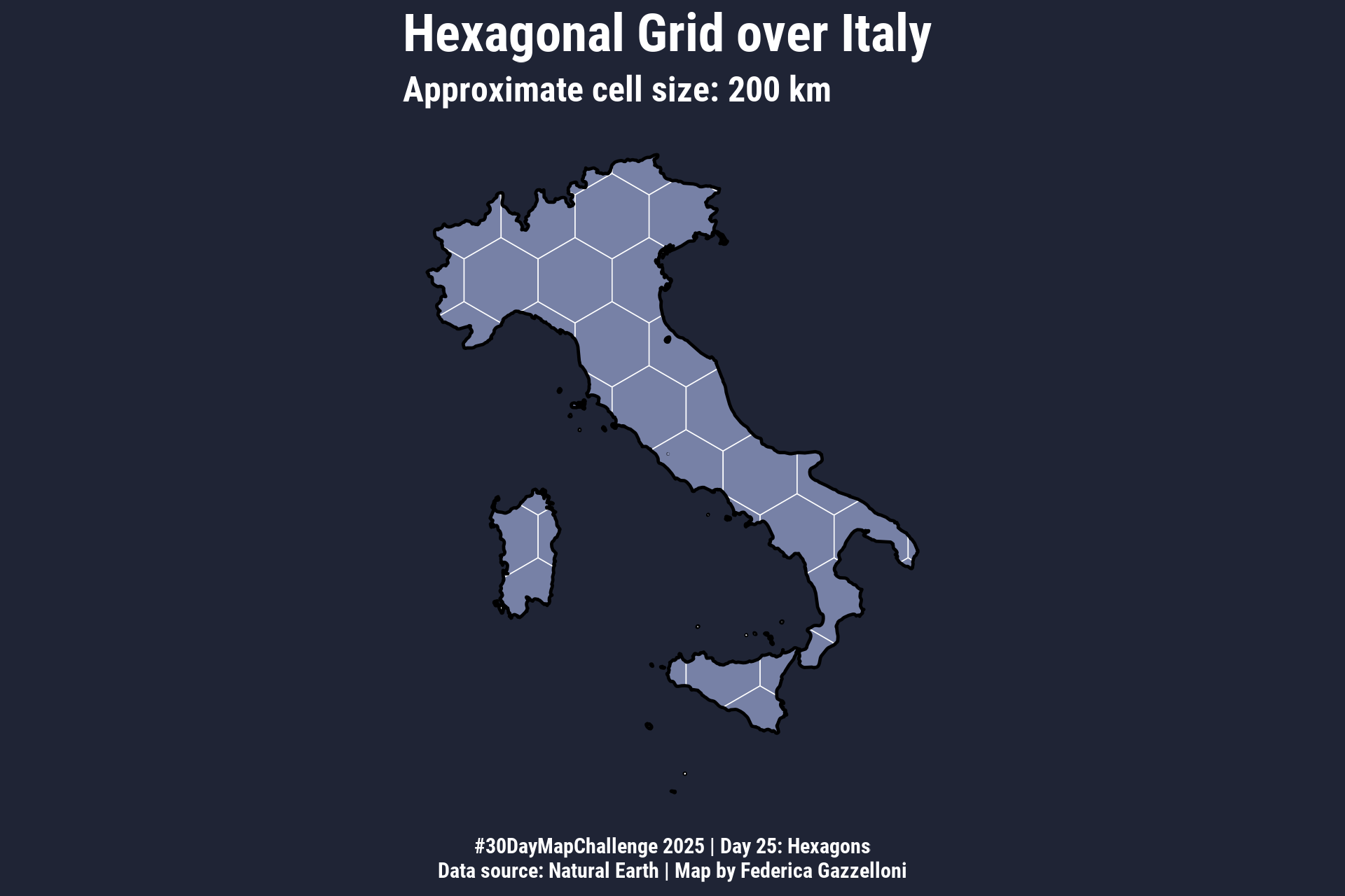
Overview
Hexagonal grids with R. We use the {sf} package.
Load Libraries
- Get Italy boundaries
# Natural Earth country boundaries
world <- rnaturalearth::ne_countries(scale = 10, returnclass = "sf")

italy <- world %>%
  filter(admin == "Italy") %>%
st_transform(3857) # good for equal-area cell grids- Create hexagonal grid (~200 km)
In EPSG:3857, metres are units → 200,000 m ≈ 200 km
square = FALSE gives hexagons
cell <- st_make_grid(
  italy,
  cellsize = 200000,    # ~200 km
  what = "polygons",
  square = FALSE         # hexagons
)

cell_sf <- st_sf(geometry = cell)- Clip hexagons to Italy
hex_it <- st_intersection(cell_sf, italy)library(showtext)
font_add_google(name = 'Roboto Condensed',
family = 'Roboto Condensed')
showtext_auto()
showtext_opts(dpi = 300)- Plot hexagonal grid over Italy
ggplot() +
  geom_sf(data = hex_it, fill = "#7781a6", color = "white") +
  geom_sf(data = italy, fill = NA, color = "black", size = 0.5) +
  ggthemes::theme_map() +
  labs(
    title = "Hexagonal Grid over Italy",
    subtitle = "Approximate cell size: 200 km",
    caption = "#30DayMapChallenge 2025 | Day 25: Hexagons\nData source: Natural Earth | Map by Federica Gazzelloni"
  ) +
  ggthemes::theme_map()+
  theme(text=element_text(color="white",
                          family="Roboto Condensed",face="bold"),
        plot.title = element_text(size = 18),
        plot.subtitle = element_text(size = 12),
plot.caption = element_text(hjust = 0.5))ggsave("day25_hexagons.png",
dpi = 320,
width = 6,
height = 4,
bg = "#1f2435")