Cell

Global Expected deaths due to Environmental Heat & Fire

Overview

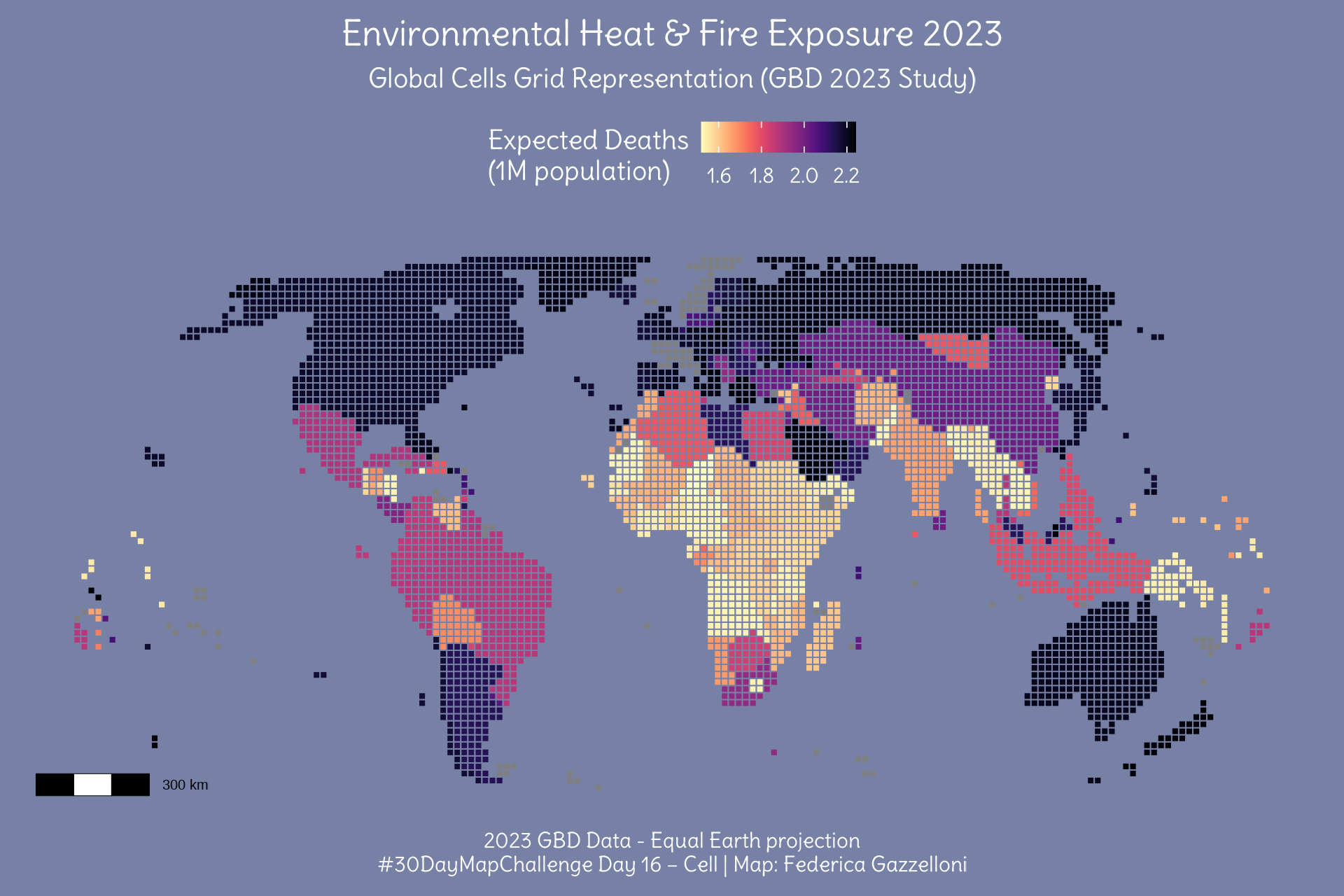
In this workflow, we generate a global map of expected deaths per 1M population due to Environmental Heat & Fire, using GBD 2023 data. We represent the world as a square grid and visualize expected values aggregated per cell.

This approach highlights geospatial patterns of exposure while keeping visual clarity at the global scale.

Load packages

library(tidyverse)
library(sf)
library(terra)

Load GBD 2023 data: Environmental Heat & Fire

Deaths per 100k due to Fire, heat, and hot substances, downloaded from the https://vizhub.healthdata.org/gbd-compare/ (you need to login first):

http://ihmeuw.org/7ana

library(readr)
raw_data <- read_csv("data/fire_heat_1.csv")
head(raw_data)

exp_deaths_data <- raw_data %>%
  select(Location, expected_value = Value, `SDI value`) %>%
  janitor::clean_names()

exp_deaths_data %>% head

Add the Countries code

code <- countrycode::countryname(exp_deaths_data$location,
                                 destination = 'iso3c') %>%
  as_tibble()%>%
  rename(code=value)
gbd <- bind_cols(code,exp_deaths_data)
gbd%>%head

Load world polygons and join GBD data

library(rnaturalearth)
world <- ne_countries(scale = "medium", returnclass = "sf") %>%
  filter(!name=="Antarctica")%>%
  st_as_sf() %>%
  select(iso_a3, name, geometry) %>%
  left_join(gbd, by = c("iso_a3" = "code"))

base_map <- ggplot() +
  geom_sf(data = world, aes(fill=sdi_value))
base_map

Transform the polygons to Equal Earth projection

world_eq <- st_transform(world, 8857) # Equal Earth projection

Make a Grid of Cells

# Cell grid (approx. 200km cells, adjust for detail)
cell <- st_make_grid(world_eq, 
                    cellsize = 200000, 
                    what = "polygons", square = T)

cell_sf <- st_sf(geometry = cell)

Joining Sets

joined <- st_join(cell_sf, world_eq, left = FALSE)

Check the base Map

base_map <- ggplot() +
  geom_sf(data = world_eq, fill = "gray90",color = "grey55",linewidth=0.2)
base_map

Set the Fots

library(showtext)
font_add_google(name = 'Delius', 
                family = 'Delius')
showtext_auto()
showtext_opts(dpi = 300)

Draw the Map

ggplot() +
  geom_sf(data = joined, aes(fill = expected_value),
          color = "#7781a6",linewidth=0.2) +
  viridis::scale_fill_viridis(option = "magma", direction = -1,
                              name = "Expected Deaths\n(1M population)",
                              labels = scales::number_format(scale = 1e2, 
                                                             accuracy = 0.1))+
  labs(title = "Environmental Heat & Fire Exposure 2023",
       subtitle = "Global Cells Grid Representation (GBD 2023 Study)",
       caption = "2023 GBD Data - Equal Earth projection\n#30DayMapChallenge Day 16 – Cell | Map: Federica Gazzelloni")+
  ggthemes::theme_map()+
  theme(text = element_text(family="Delius",
                            color="white",face="bold"),
        plot.title = element_text(size=12,hjust=0.5),
        plot.subtitle = element_text(hjust=0.5),
        plot.caption = element_text(hjust=0.5),
        plot.background = element_rect(fill="#7781a6",color=NA),
        legend.position = "top",
        legend.justification = "center",
        legend.box.just = "center",
        legend.key.size = unit(10,"pt"),
        legend.background = element_rect(fill="#7781a6")) +
    # add a dimension scale
    ggspatial::annotation_scale(
    location = "bl",      # bottom left corner
    width_hint = 0.1,     # relative width of scale bar
    text_cex = 0.4,       # text size
    line_width = 0.3,     # bar line thickness
    style = "bar"         # "ticks" for tick marks, "bar" for solid bar
  ) 

Save as png

ggsave("day16_cell.png",bg="#7781a6",
       width = 6, height = 4, dpi = 320)