Fire – Unlocking the Power of Data Visualization with R

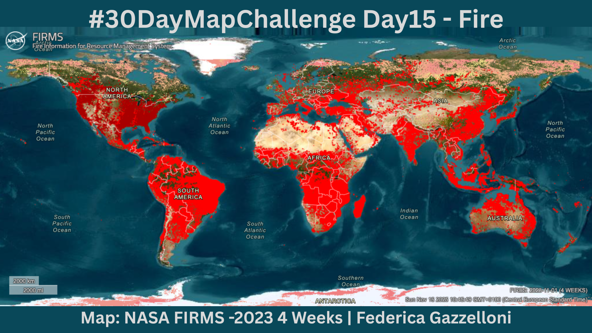
Overview

For this challenge, I explored global wildfire activity using NASA FIRMS (Fire Information for Resource Management System), an online platform that provides near real-time fire detections from MODIS and VIIRS satellites.

The map I shared was created starting from the FIRMS mapping tool, which allows interactive visualization and extraction of fire data at different temporal and spatial scales. What I find particularly valuable is the possibility to download the underlying data and integrate it into a statistical workflow for deeper analysis.

FIRMS remains one of the most accessible and powerful resources for understanding where fires occur and how patterns evolve over time. The combination of high-resolution satellite detections and user-friendly extraction tools makes it straightforward to generate maps, analyze trends, or build models.

If you work with geospatial data, climate, or public health metrics, FIRMS is an excellent starting point for reliable and up-to-date fire information.

Download FIRMS wildfire data (VIIRS 375m, year 2023)

# Create temp files
temp <- tempfile()
temp2 <- tempfile()

url <-"https://firms.modaps.eosdis.nasa.gov/data/download/DL_FIRE_J1V-C2_686477.zip"
download.file(URL, temp)
# Unzip the contents of the temp and save unzipped content in 'temp2'
unzip(zipfile = temp, exdir = temp2)
# Read the shapefile. 
fire_shp <- sf::read_sf(temp2)

# saveRDS(fire_shp,"data/fire_shp.rds")

library(data.table)
# 2. Extract coordinates as data.table (very fast)
coords_dt <- as.data.table(st_coordinates(fire_shp))
setnames(coords_dt, c("X","Y"), c("longitude","latitude"))

# 3. Optional: Save coordinates only for later use
fwrite(coords_dt, "data/VIIRS_2023_coords.csv")

coords_dt%>%head

coords_dt%>%dim

library(rnaturalearth)
world <- ne_countries(scale = "medium", returnclass = "sf") %>%
  filter(!name=="Antarctica")%>%
  st_as_sf() %>%
  select(iso_a3, name, geometry)

base_map <- ggplot() +
  geom_sf(data = world, color="grey",fill=NA)

base_map +
  geom_point(data = coords_dt,
             aes(x=longitude,y=latitude),
    color = "red",
    shape=".")

library(data.table)

unique_coords_dt <- distinct(coords_dt)

# coords_dt is already a data.table:
n <- nrow(unique_coords_dt)
s <- sample.int(n, size = floor(0.001 * n))   # 1% sample

sample_dt <- coords_dt[s]

base_map +
  geom_point(data = sample_dt,
             aes(x=longitude,y=latitude),
    color = "red",
    shape=".")

library(spatstat)
pp <- ppp(coords_dt$longitude, coords_dt$latitude, window=owin(c(-180,180),c(-90,90)))
# saveRDS(pp,"data/pp.rds")
sample_pp <- rthin(pp, P = 0.001)    # keep 1%

sample_coords2 <- as.data.frame(cbind(
  x = sample_pp$x,
  y = sample_pp$y
))

sample_sf <- st_as_sf(sample_coords2,
                      coords = c("x", "y"),
                      crs = 4326)

ggplot() +
  geom_sf(data = world) +
  geom_sf(data = sample_sf,
          fill = "darkred",
          color="grey40",
          shape=21,stroke=0.03,
          size=1, alpha=0.9)  +
  geom_sf(data = world, color="black", fill = NA)