Openstreetmap

Rome Hospitals location

Overview

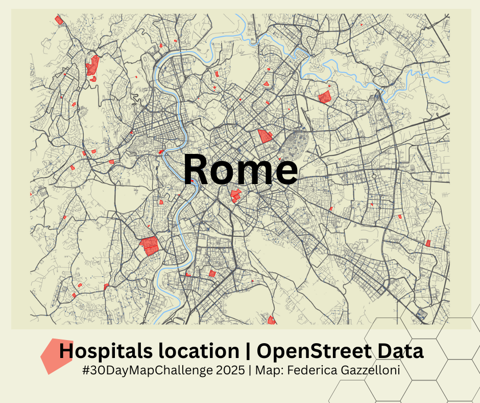
Today’s map focuses on OpenStreetMap (OSM) and the osmdata package. I wanted to build a compact visual overview of Rome by layering a few key features: highways, small streets, rivers, hospitals and bus stops. The workflow is simple, reproducible and fully based on open data.

What is expected in this type of exercise is clarity: start from a bounding box, fetch only the features you need, and build up the map step by step. Below I share the essential code blocks I used.

Get the bounding box for Rome

library(tidyverse)
library(osmdata)
library(sf)

A single call to getbb() gives you a clean area to work with:

bb <- getbb("Rome, Italy")

Download selected OSM layers

I queried a few features separately to keep things tidy and avoid timeouts:

primary <- opq(bb) %>%
  add_osm_feature("highway", c("motorway", "primary", "secondary", "tertiary")) %>%
  osmdata_sf()
# saveRDS(primary,"data/primary.rds")

secondary <- opq(bb) %>%
  add_osm_feature(key = "highway", value = c("residential", "living_street", "unclassified", "service", "footway")) %>%
  osmdata_sf()
# saveRDS(secondary,"data/secondary.rds")

rivers <- opq(bb) %>%
  add_osm_feature(key = "waterway", value = "river") %>%
  osmdata_sf()
# saveRDS(rivers,"data/rivers.rds")

# retrieving data of hospitals
hospitals <- opq(bb) %>%
  add_osm_feature("amenity", "hospital") %>%
  osmdata_sf()
# saveRDS(hospitals,"data/hospitals.rds")

# Define the bounding box of the area we want to search
bus_stops <- opq(bb) |> 
  add_osm_feature(key = "highway", value = "bus_stop") |> 
  osmdata_sf()
# saveRDS(bus_stops,"data/bus_stops.rds")

Plot with ggplot2

A layered approach helps maintain transparency and auditability:

streets <- ggplot()+
  # Add base map
  # annotation_map_tile(type = "cartolight", zoomin = 0, progress = "none") +
  geom_sf(data = primary$osm_lines,color="grey30",linewidth=0.3) +
  geom_sf(data = secondary$osm_lines,color="grey50",linewidth=0.1)
streets

streets +
  geom_sf(data = rivers$osm_lines, color="#7fc0ff") +
  geom_sf(data = hospitals$osm_polygons,color="red",fill=alpha("red",0.5)) +
  geom_sf(data= bus_stops$osm_points,shape=".", color=alpha("#3e5d8b",0.8))+
  coord_sf(xlim = c(12.4, 12.6), 
           ylim = c(41.84, 41.95), 
           expand = FALSE) +
  ggthemes::theme_map()

ggsave("base_map.png", 
       width = 6, height = 4,
       dpi =320,
       bg=alpha("#e3e4bb",0.5))