Polygons – Unlocking the Power of Data Visualization with R

Overview

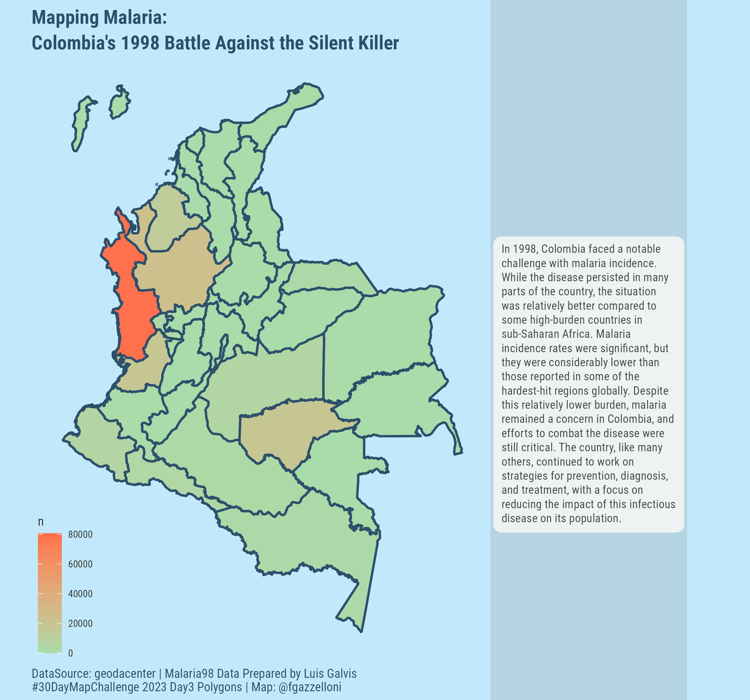
This is a map of Colombia Malaria incidence in 1998 - Data is from Geodatacenter.

library(tidyverse)
library(sf)

Useful Data-source:

Data description: https://geodacenter.github.io/data-and-lab/sids/
Vignette: https://r-spatial.github.io/spdep/articles/sids.html
More datasets: https://geodacenter.github.io/data-and-lab/

We are interested in:

Malaria in Colombia in 1998

mc <- read_sf("data/coldept.gpkg")

mc%>%names

plot(mc["MALARI98"])

mc1 <- mc["MALARI98"]
ggplot(mc1)+
  geom_sf(aes(fill=MALARI98))

text <- tibble(title=c("Mapping Malaria:\nColombia's 1998 Battle Against the Silent Killer"),
           caption=c("DataSource: geodacenter | Malaria98 Data Prepared by Luis Galvis\n#30DayMapChallenge 2023 Day3 Polygons | Map: @fgazzelloni"),
           annotation=c("In 1998, Colombia faced a notable challenge with malaria incidence. While the disease persisted in many parts of the country, the situation was relatively better compared to some high-burden countries in sub-Saharan Africa. Malaria incidence rates were significant, but they were considerably lower than those reported in some of the hardest-hit regions globally. Despite this relatively lower burden, malaria remained a concern in Colombia, and efforts to combat the disease were still critical. The country, like many others, continued to work on strategies for prevention, diagnosis, and treatment, with a focus on reducing the impact of this infectious disease on its population."))

ggplot(mc1)+
  geom_sf(aes(fill=MALARI98),color="#2D4F6B",
          linewidth=0.8)+
  scale_y_continuous(breaks = 34:36) +
  scale_fill_gradient(low = "#A8DCAA",high = "#FF704D")+
  #scale_fill_gradientn(colours = sf.colors(20)) +
  geom_segment(aes(x=-60,xend=-66,
                   y=-0.5, yend=-0.5),
               color="#b6d5e3",inherit.aes = F,
               linewidth=350)+
  ggtext::geom_textbox(data = text,
                       aes(x=-63,y=3.3,
                           label = annotation),
                         inherit.aes = F,
              size = 3, 
              family="Roboto Condensed",
              width = unit(9.5, "line"), 
              alpha = 0.9,
              color="#333333",
              fill="#f5f5f5",
              box.colour = "#f5f5f5") +
  coord_sf(clip = "off")+
  labs(title=text$title,
       caption=text$caption,
       fill="n")+
  ggthemes::theme_map()+
  theme(text=element_text(color="#333333",family = "Roboto Condensed"),
        plot.title = element_text(color="#2D4F6B",
                                  lineheight = 1.1,
                                  hjust = 0,vjust = 0.1,
                                  size=14,face = "bold"),
        plot.caption = element_text(color="#2D4F6B",
                                    hjust = 0,size=9),
        legend.background = element_blank(),
        legend.position = c(0,0))

ggsave("day3_polygons.png",
       dpi=320,
       width = 7.5,
       bg = "#C2E9FB")