# install.packages("s2")
library(sf)
sf_use_s2()
library(s2)


g = as_s2_geography(TRUE)
co = s2_data_countries()
oc = s2_difference(g, s2_union_agg(co)) # oceans
b = s2_buffer_cells(as_s2_geography("POINT(-30 52)"), 9800000) # visible half
i = s2_intersection(b, oc) # visible ocean

plot(st_transform(st_as_sfc(i), "+proj=ortho +lat_0=52 +lon_0=-30"), col = 'blue')Overview
This Dot Map comprises an overview of the EPSG Geodetic Parameter Dataset (also EPSG registry). A public registry of geodetic datums, spatial reference systems, Earth ellipsoids, coordinate transformations and related units of measurement, originated by a member of the European Petroleum Survey Group (EPSG) in 1985. (see Wikipedia)
Each entity is assigned an EPSG code between 1024 and 32767, along with a standard machine-readable well-known text (WKT) representation.
The most common is EPSG:4326 - WGS 84, latitude/longitude coordinate system based on the Earth’s center of mass, used by the Global Positioning System among others.
A map projection is a set of transformations to represent the curved two-dimensional surface of a globe on a plane. Here is a full list of all available types of projections: https://en.wikipedia.org/wiki/List_of_map_projections
All projections of a sphere on a plane are distortions of a three-dimensional surface when represented on a flat plane. These distortions arise due to the inherent differences in geometry between a three-dimensional sphere and a two-dimensional plane.
This resource shows how to make oceans: https://r-spatial.github.io/sf/articles/sf7.html
Oceans computed as the difference from the full polygon representing the entire globe:
Projections
Let’s have a look at some examples that can be used for changing the projection of a plane map, the reverse of what just said above, we are now starting from a plane surface and want to recreate a three dimensional representation of the earth.
ortho<- "+proj=ortho +lat_0=-90 +lat_ts=-71 +lon_0=0 +k=1 +x_0=0 +y_0=0 +ellps=WGS84 +datum=WGS84 +units=m +no_defs"st_transform(crs="ESRI:54030")
coord_sf(crs="ESRI:54030",clip = "off")
tm_shape(World, projection = 8857)Load necessary libraries
library(tidyverse)
library(raster)
The WorldCover_trees_30s.tif image can be downloaded here: https://geodata.ucdavis.edu/geodata/landuse/
r <- raster("data/WorldCover_trees_30s.tif")
plot(r)rr<- terra::rast(r)set.seed(27112023)
ggplot() +
tidyterra::geom_spatraster(data = rr,
aes(fill = trees)) +
coord_sf(crs = 4326,clip = "off") +
tidyterra::scale_fill_hypso_c(direction = -1)library(tmap)
data("World")
library(stars)
tif=read_stars("data/WorldCover_trees_30s.tif",
RasterIO = list(nBufXSize = 600, nBufYSize = 600))
tif_tr<-st_transform(tif,crs="ESRI:54030")sysfonts::font_add_google("Merriweather","Merriweather")
showtext::showtext_auto()
showtext::showtext_opts(dpi=320)ggplot()+
geom_stars(data=tif_tr)+
geom_sf(data=World%>%filter(!name=="Antarctica"),fill=NA,shape=".")+
coord_sf(crs = "ESRI:54030",clip = "off") +
tidyterra::scale_fill_hypso_c(direction = -1,
label=scales::percent_format(),
guide = guide_colorbar(title.position = "top"))+
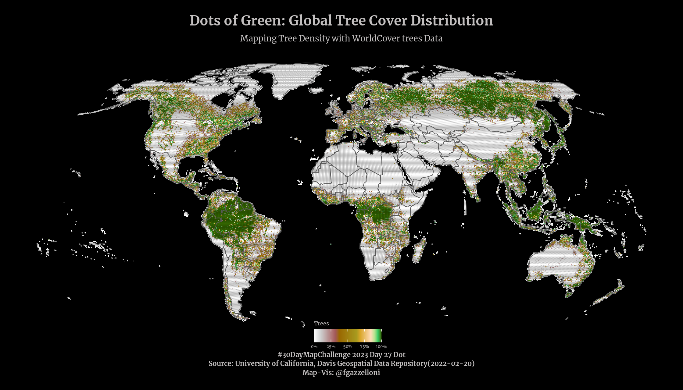
labs(title = "Dots of Green: Global Tree Cover Distribution",
subtitle=
"Mapping Tree Density with WorldCover trees Data",
caption = "#30DayMapChallenge 2023 Day 27 Dot\nSource: University of California, Davis Geospatial Data Repository(2022-02-20)\nMap-Vis: @fgazzelloni",
fill="Trees")+
ggthemes::theme_map()+
theme(text=element_text(family="Merriweather",color="#c2bfbf"),
plot.title = element_text(face="bold",size=10,hjust=0.5),
plot.subtitle = element_text(size=6,hjust=0.5),
plot.caption = element_text(face="bold",
size=5,
lineheight = 1.1,
hjust=0.5,
vjust=-0.2),
legend.text = element_text(color="#c2bfbf",size=3),
legend.title = element_text(size=4),
legend.key.size = unit(10,units = "pt"),
legend.position = c(0.45,-0.05),
legend.background = element_blank(),
legend.direction = "horizontal")ggsave("day27_dot.png",bg="black",
width = 7,
height = 4,
dpi=320)