library("tidyverse")
library("R.utils")
library("httr")
library("sf")
library("stars")
library("rayshader")Overview
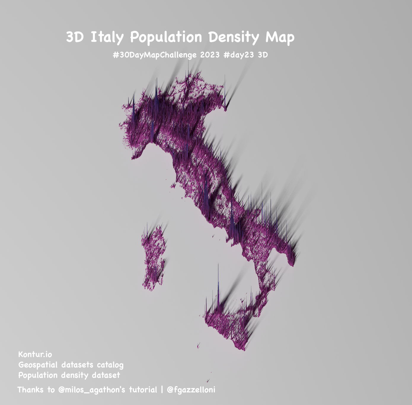
This is the 3D Italy’s Population Density Map made with the instruction provided by Milos Agathon: Milos Makes Maps tutorial:
- https://www.youtube.com/watch?v=qTDf5VVnjMM
- https://github.com/milos-agathon/making-crisp-spike-maps-with-r/blob/main/R/create-spike-map-in-r.r
Download and unzip kontur data:
url <-
    "https://geodata-eu-central-1-kontur-public.s3.amazonaws.com/kontur_datasets/kontur_population_IT_20220630.gpkg.gz"
file_name <- "italy-population.gpkg.gz"

get_population_data <- function() {
    res <- httr::GET(
        url,
        write_disk(file_name),
        progress()
    )

    R.utils::gunzip(file_name, remove = F)
}

get_population_data()
load_file_name <- gsub(".gz", "", file_name)
crsLONGLAT <- "+proj=longlat +datum=WGS84 +no_defs +ellps=WGS84 +towgs84=0,0,0"get_population_data <- function() {
pop_df <- sf::st_read(
load_file_name
) |>
sf::st_transform(crs = crsLONGLAT)
}
pop_sf <- get_population_data()
head(pop_sf)First raw image:
ggplot() +
    geom_sf(
        data = pop_sf,
        color = "grey10", fill = "grey10"
    )
# ggsave("raw.png")Make it a raster
bb <- sf::st_bbox(pop_sf)

get_raster_size <- function() {
    height <- sf::st_distance(
        sf::st_point(c(bb[["xmin"]], bb[["ymin"]])),
        sf::st_point(c(bb[["xmin"]], bb[["ymax"]]))
    )
    width <- sf::st_distance(
        sf::st_point(c(bb[["xmin"]], bb[["ymin"]])),
        sf::st_point(c(bb[["xmax"]], bb[["ymin"]]))
    )

    if (height > width) {
        height_ratio <- 1
        width_ratio <- width / height
    } else {
        width_ratio <- 1
        height_ratio <- height / width
    }

    return(list(width_ratio, height_ratio))
}
width_ratio <- get_raster_size()[[1]]
height_ratio <- get_raster_size()[[2]]

size <- 3000
width <- round((size * width_ratio), 0)
height <- round((size * height_ratio), 0)

get_population_raster <- function() {
    pop_rast <- stars::st_rasterize(
        pop_sf |>
            dplyr::select(population, geom),
        nx = width, ny = height
    )

    return(pop_rast)
}

pop_rast <- get_population_raster()
Second raw image this time as a raster:
plot(pop_rast)# ggsave("raw2.png")pop_mat <- pop_rast |>
as("Raster") |>
rayshader::raster_to_matrix()cols <- rev(c(
"#0b1354", "#283680",
"#6853a9", "#c863b3"
))
texture <- grDevices::colorRampPalette(cols)(256)Create the initial 3D object
pop_mat |>
    rayshader::height_shade(texture = texture) |>
    rayshader::plot_3d(
        heightmap = pop_mat,
        solid = F,
        soliddepth = 0,
        zscale = 15,
        shadowdepth = 0,
        shadow_darkness = .95,
        windowsize = c(800, 800),
        phi = 65,
        zoom = .65,
        theta = -30,
        background = "white"
    )
Adjust the view after building the window object
rayshader::render_camera(phi = 75, zoom = .7, theta = 0)

rayshader::render_highquality(
    filename = "italy_population_2022.png",
    preview = T,
    light = T,
    lightdirection = 225,
    lightaltitude = 60,
    lightintensity = 400,
    interactive = F,
    width = width, height = height
)