Atmosphere – Unlocking the Power of Data Visualization with R

Overview

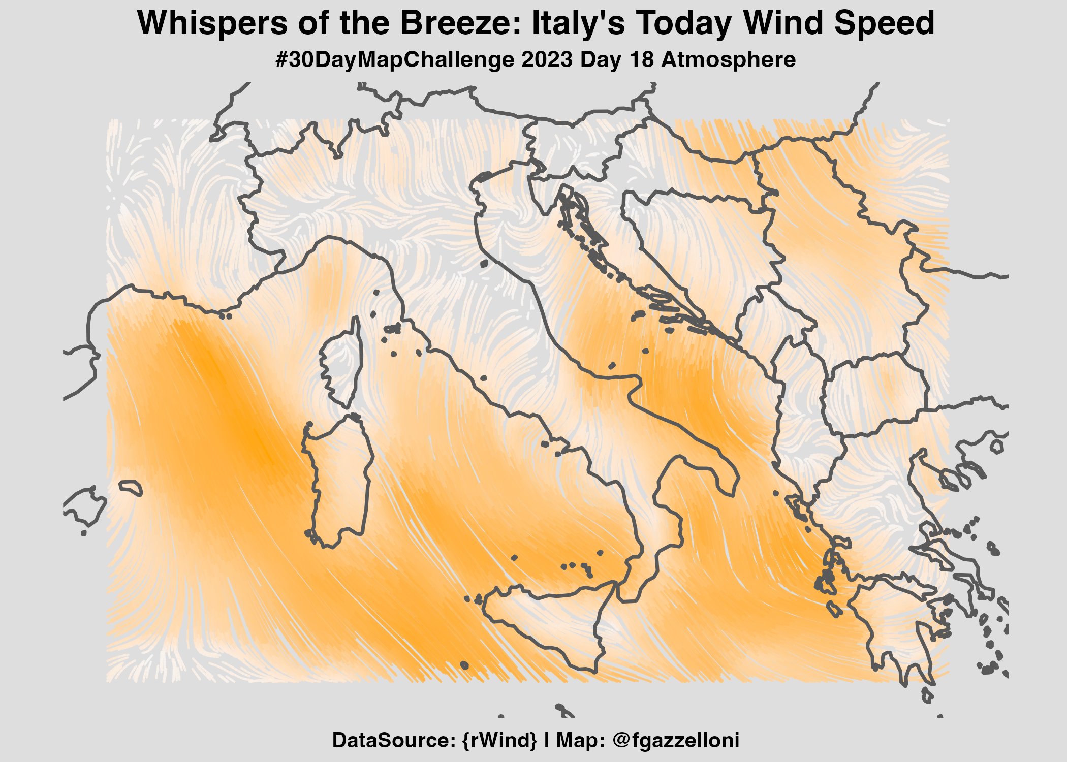
This challenge is all about wind movements. The selected area is Italy, also some parts of the surrounding territories can be seen. I am going to use the {rWind} package for downloading the information about wind speed and direction vectors (u,v) for today, Nov 18, 2023.

In order to be able to interpolate the information from {rWind}, I’ll use the {oce} package which provide a type of interpolating function for calculating the Barnes interpolation with: oce::interpBarnes() function.

Load necessary libraries

library(tidyverse)
library(sf)
library(giscoR)
library(classInt)
library(metR)
# devtools::install_github("jabiologo/rWind")
# install.packages("oce")
library(rWind)
library(oce)

Set the Date

time_range <- seq(ymd_hms(paste(2023, 11, 18, 00, 00, 00, 
                                sep = "-")),
                  ymd_hms(paste(2023, 11, 18, 00, 00, 00, 
                                sep = "-")),
                  by = "1 hours"
                  )

Download Data from {rWind}

mean_wind_data2 <- rWind::wind.dl_2(time_range, 
                                   3.472, 36.368, 23.906, 46.665) %>%
  rWind::wind.mean()

eur_wind_df2 <- as.data.frame(mean_wind_data2)
eur_wind_df2%>%head

Quick look at the first grid

ggplot(eur_wind_df2)+
  geom_point(aes(lon,lat,color=speed),size=1.5,alpha=0.9)

Download the polygons for Europe

eur_sf <- giscoR::gisco_get_countries(
        year = "2020", epsg = "4326",
        resolution = "10", region = c("Europe", "Asia")
    )

Have a look at the first level map

ggplot(eur_wind_df2)+
  geom_point(aes(lon,lat,color=speed),size=2)+
  geom_sf(data=eur_sf,inherit.aes = F,
          fill=NA,
          show.legend = F)+
  scale_color_gradient(low="#f6f7f9",high = "#250c5f")+
  scale_x_continuous(limits = c(3.472,23.906))+
  scale_y_continuous(limits = c(36.368,46.665))+
  theme(panel.background = element_rect(color="#f6f7f9",fill="#f6f7f9"))

Interpolation

Here I try to make the Barnes interpolation on the first level grid.

oce::interpBarnes

And have a look at the information provided with the contour() function.

wu <- oce::interpBarnes(
        x = eur_wind_df2$lon,
        y = eur_wind_df2$lat,
        z = eur_wind_df2$ugrd10m
    )
wv <- oce::interpBarnes(
        x = eur_wind_df2$lon,
        y = eur_wind_df2$lat,
        z = eur_wind_df2$vgrd10m
    )
contour(wu$xg,wu$yg,wu$zg)

Set a second level grid

eur_wind_pts <- eur_wind_df2 %>%
    sf::st_as_sf(coords = c("lon", "lat")) %>%
    sf::st_set_crs(4326)

eur_wind_pts

 eur_wind_grid <- eur_wind_pts %>%
    sf::st_make_grid(n = c(80, 100)) %>%
    sf::st_sf() %>%
    dplyr::mutate(id = row_number())

Have a look at the second level grid

ggplot(eur_wind_grid)+
  geom_sf()

Make an adjusted grid set

For more information about this type of analysis have a look at this tutorial: https://milospopovic.net/mapping-wind-data-in-r/

eur_wind_grid_agg <- 
    sf::st_join(eur_wind_pts, eur_wind_grid, 
      join = sf::st_within) %>%
    sf::st_drop_geometry() %>%
    dplyr::group_by(id) %>%
    dplyr::summarise(
      n = n(), u = mean(ugrd10m), 
      v = mean(vgrd10m), speed = mean(speed)
    ) %>%
    dplyr::inner_join(eur_wind_grid, by="id") %>%
    dplyr::select(n, u, v, speed, geometry) %>%
    sf::st_as_sf() %>%
    na.omit()

Visualize the adjusted grid

ggplot(eur_wind_grid_agg)+
  geom_sf(aes(fill=speed))

Rebuild the original set with adding adjusted coordinates

The Centroids:

coords <- eur_wind_grid_agg %>%
    st_centroid() %>%
    st_coordinates() %>%
    as_tibble() %>%
    rename(lon = X, lat = Y)

eur_df <- coords %>%
    bind_cols(sf::st_drop_geometry(eur_wind_grid_agg))

eur_df %>%
        ggplot() +
        geom_point(aes(lon,lat,color=speed))

Interpolation II

Repete the procedure with the adjusted grid.

wu <- oce::interpBarnes(
        x = eur_df$lon,
        y = eur_df$lat,
        z = eur_df$u
    )

dimension <- data.frame(lon = wu$xg, wu$zg) %>% dim()

udf <- data.frame(
        lon = wu$xg,
        wu$zg
    ) %>%
        gather(key = "lata", value = "u", 2:dimension[2]) %>%
        mutate(lat = rep(wu$yg, each = dimension[1])) %>%
        select(lon, lat, u) %>%
        as_tibble()

wv <- oce::interpBarnes(
        x = eur_df$lon,
        y = eur_df$lat,
        z = eur_df$v
    )

vdf <- data.frame(lon = wv$xg, wv$zg) %>%
        gather(key = "lata", value = "v", 2:dimension[2]) %>%
        mutate(lat = rep(wv$yg, each = dimension[1])) %>%
        select(lon, lat, v) %>%
        as_tibble()

df <- udf %>%
        bind_cols(vdf %>% select(v)) %>%
        mutate(vel = sqrt(u^2 + v^2))

head(df)

Make the Map

df %>%
        ggplot() +
        metR::geom_streamline(
            data = df,
            aes(
                x = lon, y = lat, dx = u, dy = v,
                color = sqrt(..dx..^2 + ..dy..^2)
            ),
            L = 2, res = 2, n = 60,
            arrow = NULL, lineend = "round",
            alpha = .85
        )

Make the map on polygons

df %>%
  ggplot() +
  metR::geom_streamline(data = df,
                        aes(x = lon, y = lat, dx = u, dy = v,
                            color = sqrt(..dx..^2 + ..dy..^2)),
                        L = 2, 
                        res = 2, 
                        n = 60,arrow = NULL, 
                        lineend = "round",
                        alpha = .85) +
  geom_sf(data = eur_sf,
          fill = NA,
          linewidth = 0.8,
          alpha = .99) +
    scale_x_continuous(limits = c(3.472,23.906))+
    scale_y_continuous(limits = c(36.368,46.665))+
  scale_color_gradient(low="#f6f7f9",high = "orange")+
  labs(title="Whispers of the Breeze: Italy's Today Wind Speed",
       subtitle="#30DayMapChallenge 2023 Day 18 Atmosphere",
       caption="DataSource: {rWind} | Map: @fgazzelloni")+
  ggthemes::theme_map()+
  theme(legend.position = "none",
        plot.background = element_rect(color="#dedede",fill="#dedede"),
        plot.title = element_text(hjust=0.5,size=16,face="bold"),
        plot.subtitle = element_text(hjust=0.5,size=11,face="bold"),
        plot.caption = element_text(hjust=0.5,size=10,face="bold"))

ggsave("day18_atmosphere.png",
       height = 5,
       bg="#dedede")