Oceania – Unlocking the Power of Data Visualization with R

Overview

This map of Oceania shows Population Peaks of Oceania’s Cities.

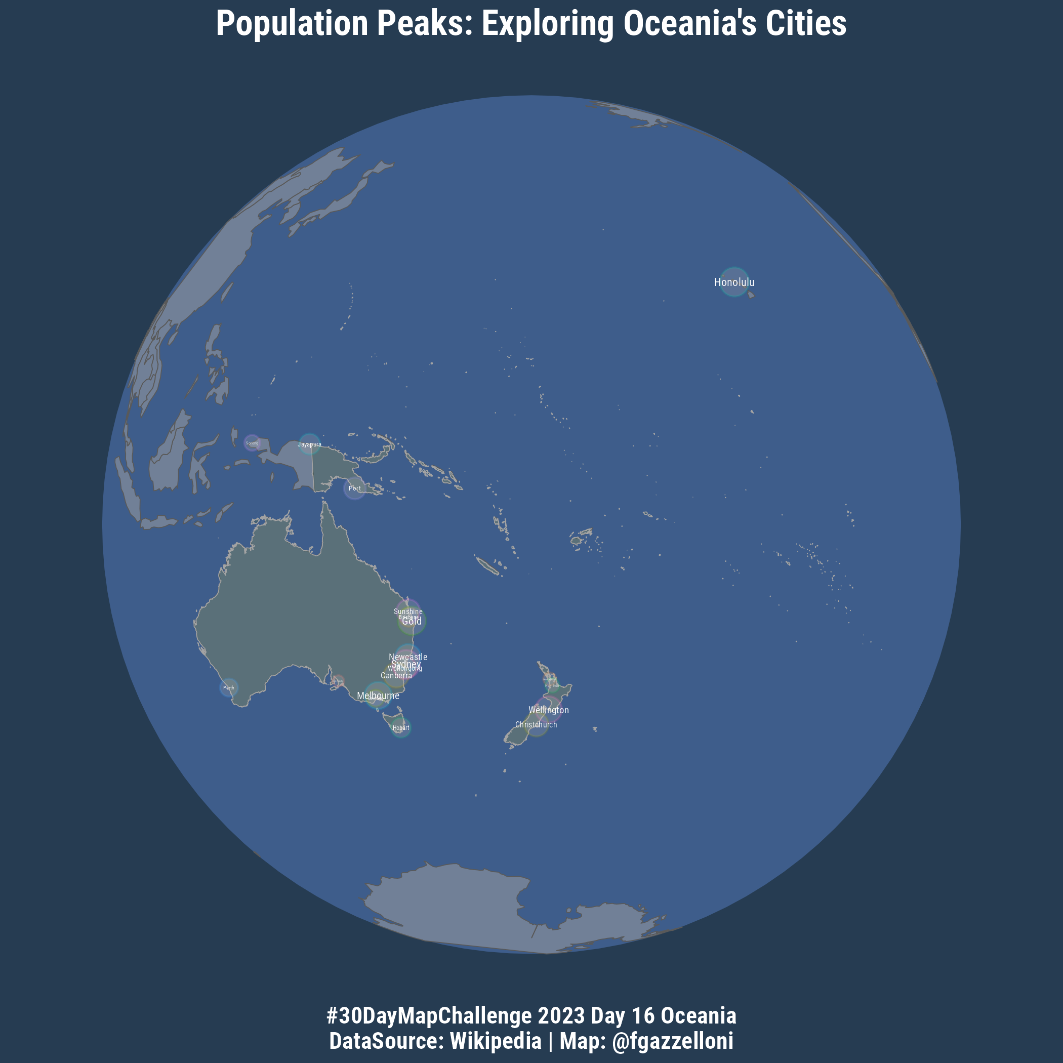
Oceania is divided into:

Australasia (largest city: Sydney)
Melanesia (largest city: Jayapura)
Micronesia (largest city: Tarawa)
Polynesia (largest city: Honolulu)

Data is scraped from Wikipedia: https://en.wikipedia.org/wiki/Oceania

Load necessary libraries:

library(tidyverse)
library(rvest)
library(ggmap)
library(sf)
library(rnaturalearth)

oceania <- read_html("https://en.wikipedia.org/wiki/Oceania")

oceania %>%
  html_nodes("table") %>%
  .[[2]] %>%
  html_table(fill = TRUE)

oceania_rank <- oceania %>%
  html_nodes("table") %>%
  .[[3]] %>%
  html_table(fill = TRUE,header = F)

# distinct(oceania_rank[-c(1,2),1])
# distinct(oceania_rank[-c(1,2),10])
oceania_rank_tb <- oceania_rank[-c(1,2),-c(1,10)]
names(oceania_rank_tb) <- oceania_rank[2,-c(1,10)]%>%unlist()
oceania_rank_tb <- rbind(oceania_rank_tb[1:4],oceania_rank_tb[5:8])%>%
  drop_na()%>%
  janitor::clean_names()

city.geo <- geocode(oceania_rank_tb$city_name)

oceania_city.geo <- cbind(oceania_rank_tb,city.geo)%>%
  mutate(city_name=gsub("[, ].*$","",city_name))

worldmap <- ne_countries(scale = 'large', type = 'map_units',
                         returnclass = 'sf')
# have a look at these two columns only
head(worldmap[c('name', 'continent')])

oceania_basemap <- worldmap[worldmap$continent == 'Oceania',]
ggplot() + 
  geom_sf(data = oceania_basemap) + 
  coord_sf(crs='ESRI:54009')

ggplot() + 
  geom_sf(data = oceania_basemap) + 
  coord_sf( crs= "+proj=ortho +lat_0=-25 +lon_0=120")

oceania_city.geo_sf<- oceania_city.geo%>%
  st_as_sf(coords = c("lon","lat"),crs="EPSG:4326")

ggplot() + 
  geom_sf(data = oceania_basemap) + 
  geom_sf(data=oceania_city.geo_sf,
          mapping=aes(size=pop),
          shape=21,stroke=0.5,show.legend = F)+
  coord_sf(crs= "+proj=ortho +lat_0=-25 +lon_0=120")+
  ggthemes::theme_map()

ortho<- "+proj=ortho +lat_0=-15.736352 +lon_0=171.740558"
ocean <- st_point(x = c(0,0)) %>%
  st_buffer(dist = 6371000) %>% #6,371km ratius of the earth
  st_sfc(crs = ortho)

oceania_city.geo_sf_coords <- oceania_city.geo_sf%>%
  sf::st_coordinates()%>%
  cbind(oceania_city.geo_sf)

library(tmap)
data("World")
plot(World)

#devtools::install_github("signaux-faibles/rsignauxfaibles")
library(rsignauxfaibles)

oceania_city.geo%>%
  count(city_name)

city.colors <- rep(RColorBrewer::brewer.pal(10,"Set3"),2)

ggplot() + 
  geom_sf(data = ocean, 
          fill = "#3e5d8b", 
          color = "#263c52") + #grey34
  geom_sf(data = World,fill="grey64",alpha=0.5) + 
  geom_sf(data = oceania_basemap,
          fill="#43605b",color="grey64",
          alpha=0.5) + 
  geom_sf(data=oceania_city.geo_sf,
          mapping=aes(size=pop,color=city_name),
          fill="grey",
          #color="grey34",
          alpha=0.2,
          shape=21,stroke=0.7,
          show.legend = F)+
  scale_size_discrete()+
  ggnewscale::new_scale(new_aes = "size")+
  geom_sf_text(data=oceania_city.geo_sf_coords,
            mapping=aes(x=X,y=Y,label=city_name,size=pop), 
            nudge_x = c(0, .15, rep(0, 10), 0, 0),
            nudge_y = c(0, -.2, rep(0, 10), -.15, 0),
            fun.geometry = sf::st_centroid,
            #size=1.9,
            color="white",
            face="bold",
            family="Roboto Condensed")+
  scale_size_manual(values=seq(0.5,2,0.075))+
  coord_sf(crs= ortho)+
  labs(title="Population Peaks: Exploring Oceania's Cities",
       caption = "#30DayMapChallenge 2023 Day 16 Oceania\nDataSource: Wikipedia | Map: @fgazzelloni")+
  ggthemes::theme_map()+
  theme(text=element_text(family = "Roboto Condensed",face="bold",size=14,color="white"),
        plot.title = element_text(hjust=0.5),
        plot.caption = element_text(hjust=0.5),
        legend.position = "none")

ggsave("day16_oceania.png",bg="#263c52")

Overview

References