library(tidytuesdayR)
library(tidyverse)
library(showtext)
library(ggtext)
library(scales)
library(extrafont)
library(patchwork)
library(cowplot)
library(ragg)
library(rmarkdown)
library(hrbrthemes)
library(wesanderson)Overview
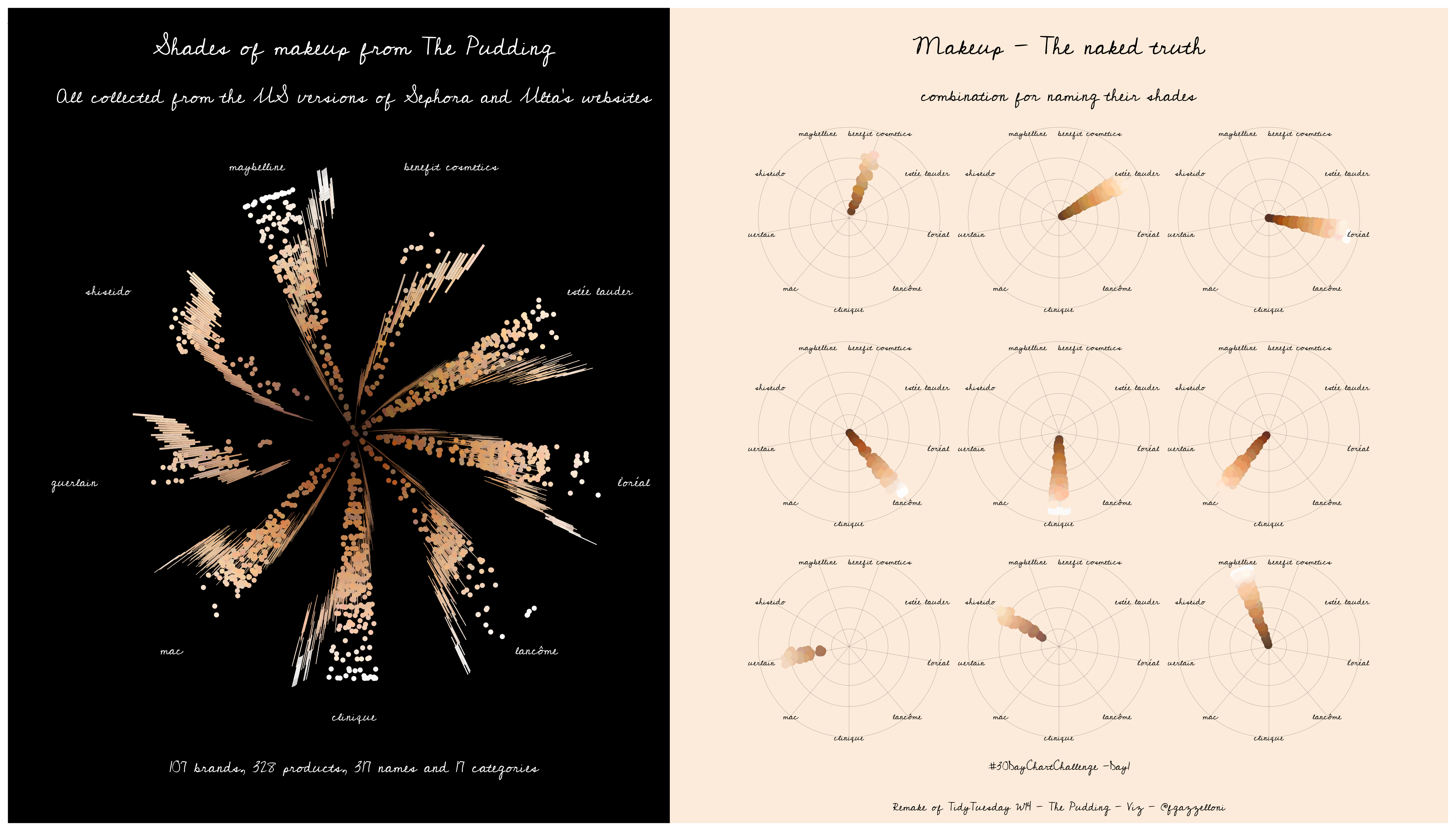
This is the first plot I made for TidyTuesday W14 - 2021 edition, based on The Pudding Data about makeup shades collected from Sephora and Ulta websites.
It shows the distribution of lightness of makeup shades for some of the most popular brands, using a polar coordinate system.
Load libraries
Load Datasets
sephora <- readr::read_csv('https://raw.githubusercontent.com/rfordatascience/tidytuesday/master/data/2021/2021-03-30/sephora.csv')
ulta <- readr::read_csv('https://raw.githubusercontent.com/rfordatascience/tidytuesday/master/data/2021/2021-03-30/ulta.csv')

allCategories <- readr::read_csv('https://raw.githubusercontent.com/rfordatascience/tidytuesday/master/data/2021/2021-03-30/allCategories.csv')
allShades <- readr::read_csv('https://raw.githubusercontent.com/rfordatascience/tidytuesday/master/data/2021/2021-03-30/allShades.csv')
allNumbers <- readr::read_csv('https://raw.githubusercontent.com/rfordatascience/tidytuesday/master/data/2021/2021-03-30/allNumbers.csv')
Load fonts
loadfonts()
font_add_google(name = "Amatic SC", family = "amatic-sc")
font_add_google("Cedarville Cursive", "cedarville")

showtext_auto(enable = TRUE)

palette <- c("#FF0000","#FF7070",
             "#F09200","#FFBF1F","#00A08A",
             "#2989A3","#5BBCD6","#A475D9")
Manipulation of data
sephora_sub<-sephora%>%
  mutate(shop=rep("sephora",length(brand)),
         brand=tolower(brand),
         product=tolower(product),
         name=tolower(name))%>%
  select(brand,product,name)

ulta_sub<-ulta%>%
  mutate(shop=rep("ulta",length(brand)),
         brand=tolower(brand),
         product=tolower(product),
         name=tolower(name))%>%
  select(brand,product,name)


shops<-rbind(sephora_sub,ulta_sub)
Manipulation of data
allCategories_sub<-allCategories%>%
  mutate(brand=tolower(brand),
         product=tolower(product),
         name=tolower(name))%>%
  separate_rows(categories, convert = TRUE) %>%
  mutate(categories = fct_reorder(categories, lightness))  %>%
  select(brand,product,name,hex,lightness,categories)

allShades_sub<-allShades%>%
  mutate(brand=tolower(brand),
         product=tolower(product),
         name=tolower(name))%>%
  select(brand,product,name,hex,hue,sat,lightness)

allNumbers_sub<-allNumbers%>%
  mutate(brand=tolower(brand),
         product=tolower(product),
         name=tolower(name))%>%
  select(brand,product,name,hex,lightness,lightToDark)
################### Full Join of the datasets ##############
make_up<-full_join(allCategories_sub,
allShades_sub)
make_up<-full_join(make_up,allNumbers_sub)
make_up_sub<-make_up%>%
select(brand,name,hex,hue,sat,lightness)%>%
filter(!is.na(hue))%>%
arrange(hex)Counting uniqueness
plyr::count(make_up$brand); #107
plyr::count(make_up$product);#328
plyr::count(make_up$name);#1,317
plyr::count(allCategories_sub$categories)#17
Selection of data for making plots
my_companies <- sort(c("shiseido","maybelline",
                       "mac","lancôme","l'oréal",
                       "guerlain","estée lauder",
                       "clinique","benefit cosmetics"),
                     decreasing = TRUE)

make_up_for_plot <- make_up_sub %>%
  filter(brand %in% my_companies) %>%
  select(brand, name,hex, hue,sat,lightness) %>%
  mutate(brand=as.factor(brand)) %>%
  group_by(brand) %>%
  mutate(mean_lightness = mean(lightness)) %>%
  ungroup() %>%
mutate(brand = fct_reorder(brand, mean_lightness))library(ggfx)
library(gridExtra)
plot1<-make_up_for_plot%>%
ggplot(aes(brand,lightness,col=hex)) +
with_blur(
geom_boxplot(size=5,show.legend = FALSE)) +
geom_jitter(width = 0.15,height = 0.0,size = 1) +
scale_colour_identity() +
coord_polar() +
labs(title = "Shades of makeup from The Pudding",
subtitle = "All collected from the US versions of Sephora and Ulta’s websites",
caption = "107 brands, 328 products, 317 names and 17 categories",
tag = "The Pudding",
x = "Lightness",
y = "Brands)",
colour = "white")+
theme_void(base_family = "cedarville") +
theme(plot.background = element_rect(fill = "black",color="black"),
axis.text.x = element_text(size = 30, vjust = 2,color="white"),
plot.title = element_text(size = 56,hjust = 0.5,color="white"),
plot.subtitle = element_text(size = 46,hjust = 0.5,color="white"),
plot.caption = element_text(size = 36,hjust = 0.5,
margin = margin(t = 5, b = 10),color="white"),
plot.tag = element_text()
)
plot2<-make_up_for_plot%>%
ggplot(aes(brand,lightness,col=hex)) +
with_blur(
geom_point(show.legend = FALSE)) +
geom_jitter(width = 0.15,height = 0.0,size = 2) +
scale_colour_identity() +
coord_polar(direction=1) +
theme_void() +
theme(plot.background = element_rect(fill = "black")) +
facet_wrap(vars(brand))Final plot
library(ggimage)
require(magick)


main_plot <- plot1 + plot2

final <- main_plot +
  labs(title = "Makeup - The naked truth",
       subtitle = "combination for naming their shades",
       caption = "#30DayChartChallenge -Day1\nRemake of TidyTuesday W14 - The Pudding - Viz - @fgazzelloni") +
  scale_fill_manual(values = palette,
                    guide = guide_legend(title = NULL)) +
  theme_void(base_family = "cedarville") +
  theme(plot.background = element_rect(fill = "#FCEBDA",color = NA),
        strip.text.x = element_text(color = NA),
        axis.text.x = element_text(size = 20, vjust = 2),
        panel.grid.major = element_line(size = 0.03, linetype = 'solid',colour = "black"),
        plot.margin = margin(10, 10, 5, 10),
        plot.title = element_text(size = 56,hjust = 0.5, margin = margin(t = 5, b = 10)),
        plot.subtitle = element_text(size = 40,hjust = 0.5),
        plot.caption = element_text(hjust = 0.5, size = 26))
Save the plot in a .png file
ragg::agg_png("day1_part-to-whole.png",
              res = 320, width = 14,
              height = 8, units = "in")
final

dev.off()