Chapter 2 Machine Learning tools
2.1 K-Nearest Neighbors (KNN)
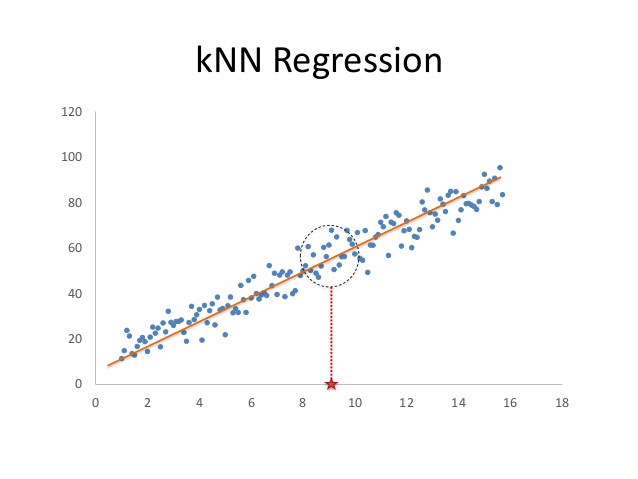
kNN is a simple and very useful method, in which predictions are made taking into account the values of the closest instances of the new COVID-19 number of cases to be predicted. In this way, the distance of all the neighbors to the new instance is computed and from there the number of neighbors considered is selected. Likewise, in this model it is vitally important to normalize the data so that one variables do not become more important than others due solely to the differences between their magnitudes. In the case of regression, the new instance is assigned the mean value of the selected neighboring instances. This algorithm usually works best when we don’t have a large number of variables.
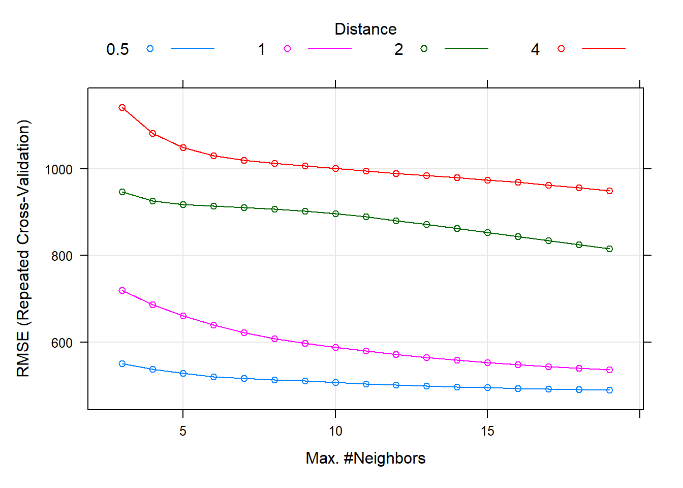
In this way, the following hyperparameters have been optimized for the implemented KNN algorithm:
kmax: Number of K-neighborsDistance: In this case, the Minkowski distance with \(p = 0.5\).kernel: best kernel to get the distances of the neighbors.
And after the iterative process of searching for hyperparameters, it has been obtained that the best values for them are the following (Likewise, we must mention that the RMSE and MAE obtained in the training have very high values, although it is also for a greater number of samples than for the test.):
| kmax | distance | kernel | RMSE | Rsquared | MAE | RMSESD | RsquaredSD | MAESD |
|---|---|---|---|---|---|---|---|---|
| 19 | 0.5 | optimal | 489.8482 | 0.7534109 | 252.2073 | 112.3373 | 0.0983198 | 52.23981 |
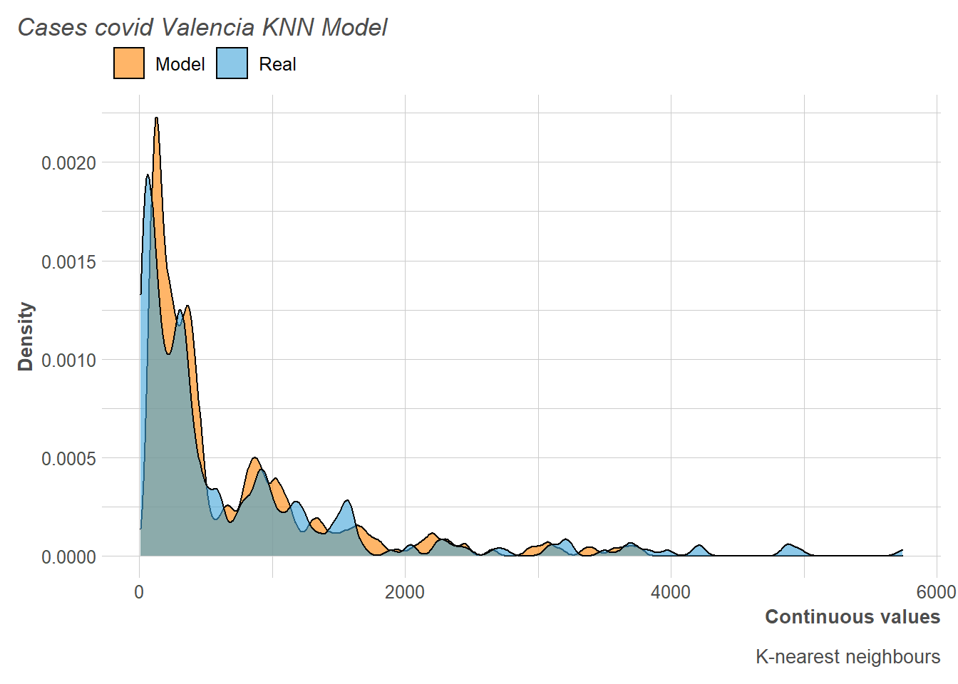
Next, we can observe the distribution of the numbers of COVID-19 cases in Valencia compared to those predicted by the model in the training session. In this way, it can be seen how our model ends up giving slightly higher predictions that will then be reflected in the selected metrics.
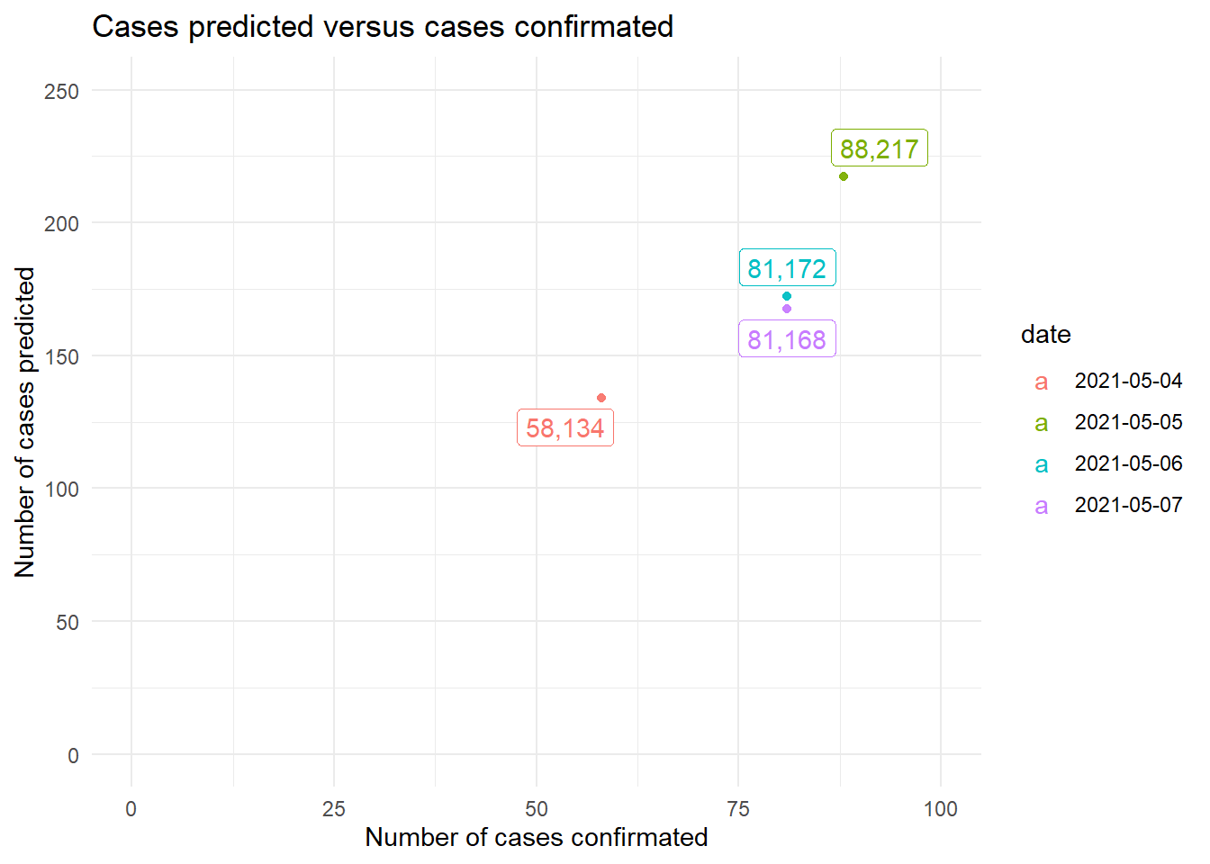
On the other hand, when viewing the predictions made in the test observations against such observations, it is appreciated that, clearly, the KNN has a tendency to increase the number of COVID-19 cases per day.
Finally, the root mean square error (RMSE) and the mean absolute error (MAE) have given excessively high values, so we could say that the KNN algorithm is not the best to perform this regression.
| RMSE |
|---|
| 97.83699 |
| MAE |
|---|
| 95.75181 |
2.2 Support Vector Machines (SVM)
Support Vector Machines are powerful and versatile machine learning models, capable of performing both linear and non-linear regression. This type of model aims to solve the optimization problem in which you want we want to minimize the error up to some degree \(\epsilon\).Thus, the instances that define the margins of each class are called support vectors. Thus, this model works especially in small or medium-sized data sets, so a good prediction result would be expected.
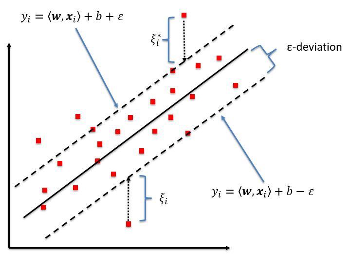
Likewise, to perform a non-linear regression, SVMs use the kernel trick, from which it is possible to achieve the same result as if multiple polynomial characteristics had been added in order to find a better minimization of the error. It should be noted that these types of models are sensitive to the characteristic scales, so it is necessary to scale them in order to obtain a good decision limit.
2.2.1 SVM with linear kernel
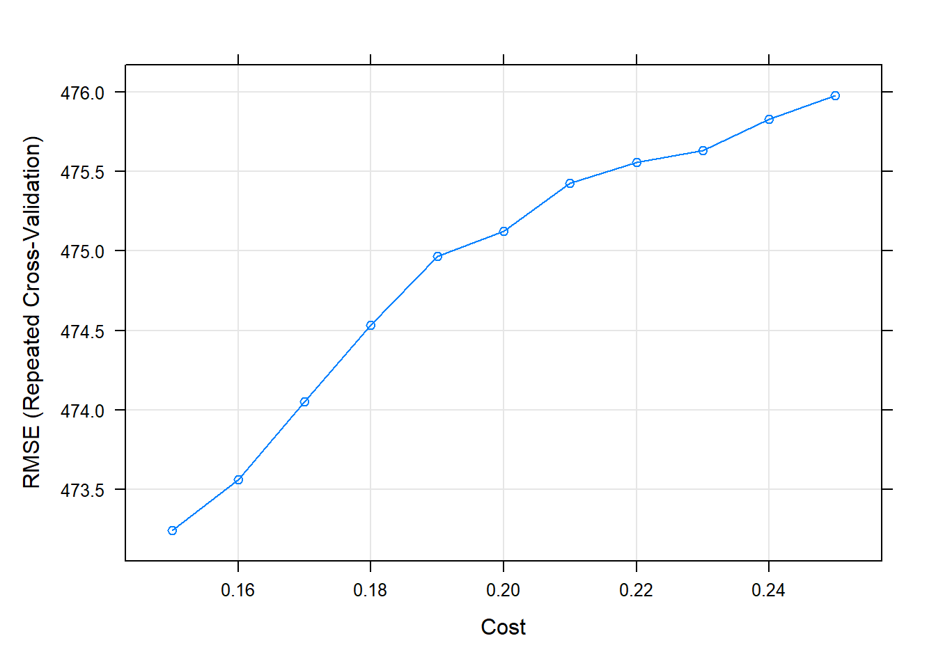
To obtain good results with this model, the hyper-parameter C has been optimized, which controls the regularization of the model. Thus, a smaller C value will give us a model with a higher bias but a lower variance (more underfitted) while a model with a higher C will give us a model with a lower bias but a higher variance (more overfitted).
Thus, after train and validate the model, it has been obtained that the best model is with \(C = 0.25\), since it is with the one that obtains the best root mean square error (RMSE), which again very high and also the MAE.
# best parameters and results of the best model
knitr::kable(get_best_result(svml_tune_v1), align = "c", "simple")| C | RMSE | Rsquared | MAE | RMSESD | RsquaredSD | MAESD |
|---|---|---|---|---|---|---|
| 0.15 | 473.2425 | 0.7596841 | 254.2694 | 62.71362 | 0.0705367 | 27.90042 |
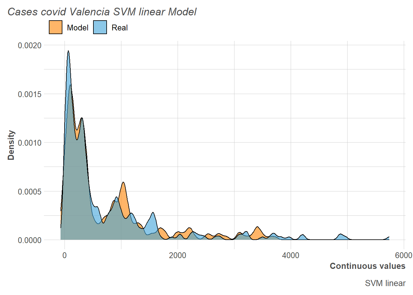
Next we observe how, although it is true that the peak of the distribution is taken very well by the model, then several alternations occur that negatively affect the metrics obtained.
On the other hand, when observing the results in the test, it is appreciated that the number of daily cases of COVID-19 is clearly overestimated.
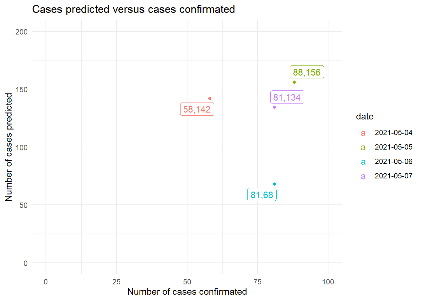
Finally, we can see how the results of the RMSE and MAE metrics regarding the test are still very high.
| RMSE |
|---|
| 60.54546 |
| MAE |
|---|
| 54.54168 |
2.2.2 SVM with gaussian kernel
In this case, two hyperparameters must be optimized: C and sigma. Both influence the regularization of the model and, having to optimize two hyper-parameters instead of one, turns out to be a more computationally expensive method. Also, it should be noted that this method can be implemented thanks to the kernel trick mentioned above.
Thus, the results of the optimization and the search of the hyperparameters have been the following, in which it can be seen how the RMSE and MAE are very high.
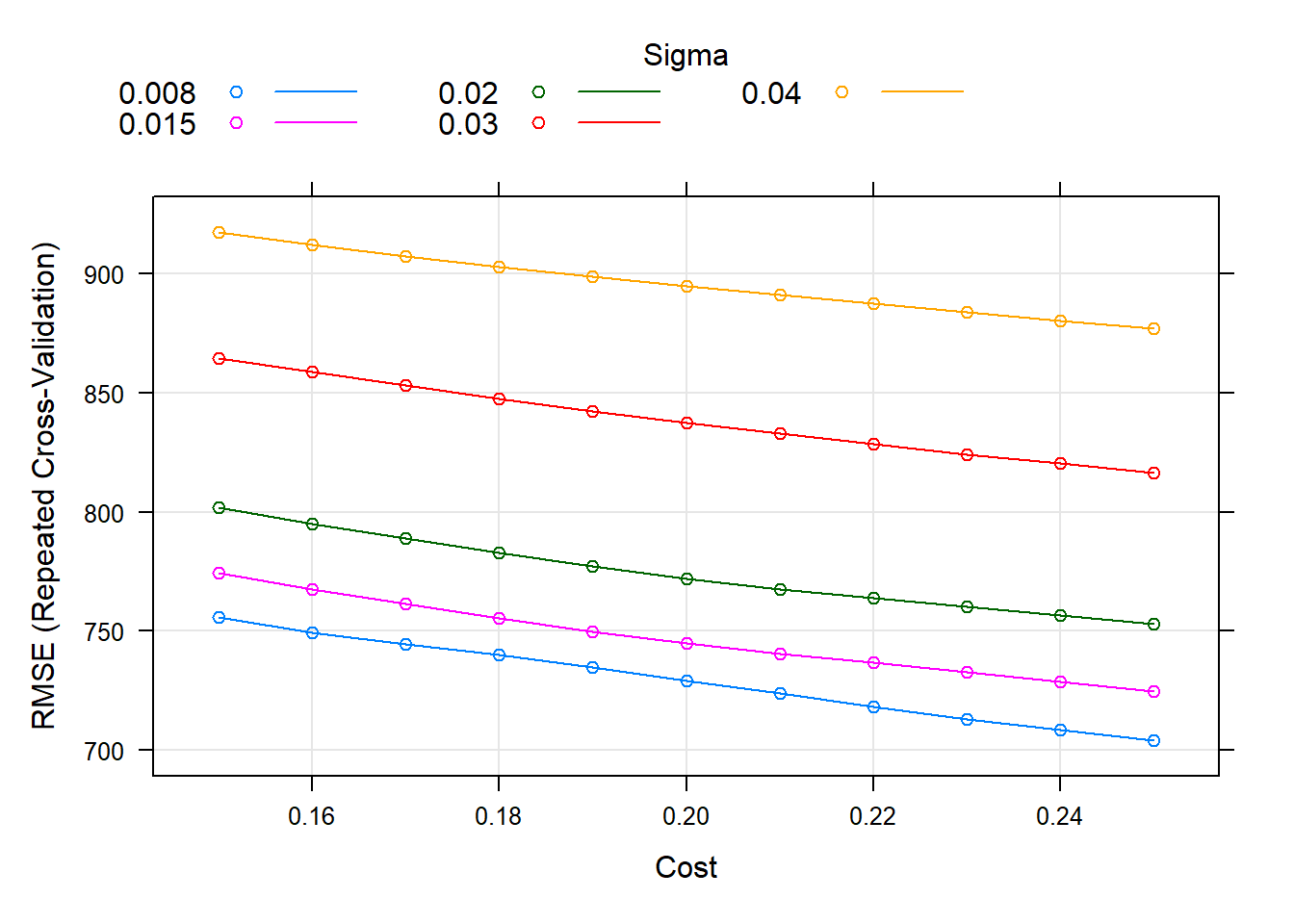
# best parameters and results of the best model
knitr::kable(get_best_result(svmr_tune_v1), align = "c", "simple")| C | sigma | RMSE | Rsquared | MAE | RMSESD | RsquaredSD | MAESD |
|---|---|---|---|---|---|---|---|
| 0.25 | 0.008 | 703.9787 | 0.6899279 | 351.7112 | 136.8075 | 0.0576779 | 73.70914 |
Regarding the distribution of the number of cases predicted by the model with the training data, this time it is observed as slightly underestimate, and the distribution itself is also slightly shifted to the left.
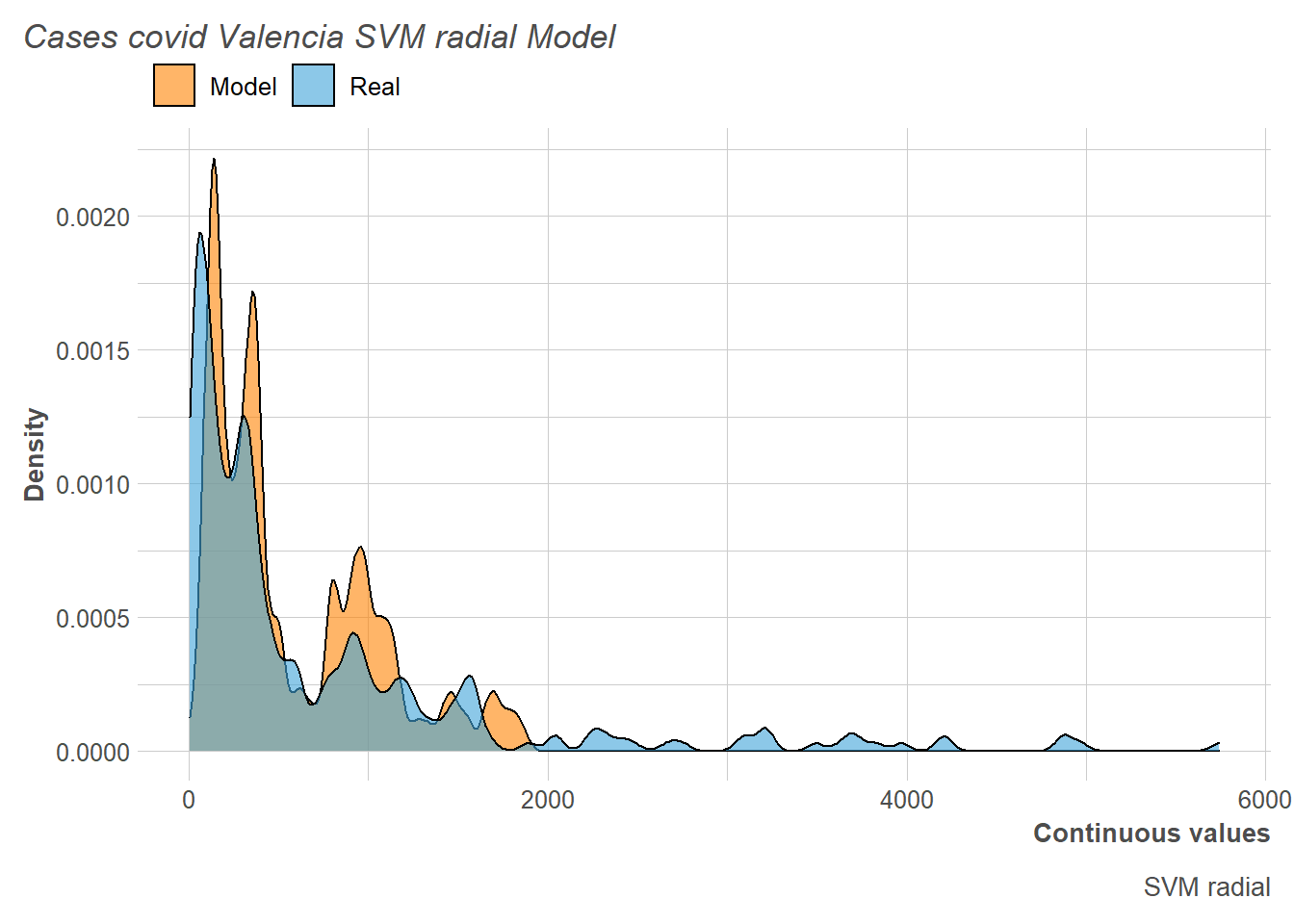
However, when analyzing the results with respect to the test, it can be seen how the model predicts more number of cases than there will be. This gives us a clue to the data that we are trying to predict, i.e, since this is a period where Valencia has had very few confirmed cases, the model over-fits based on previous experience (training set).
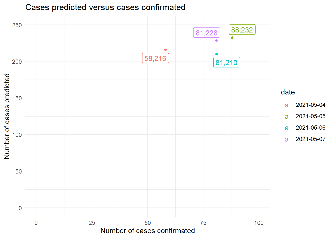
| RMSE |
|---|
| 144.9842 |
| MAE |
|---|
| 144.6181 |
Consequently, we obtain a very high RMSE and MAE to give a positive assessment to the results of the model.
2.3 Decision Trees (DT)
Decision trees are very simple models that are very useful today. One of its main advantages compared to other types of models is its great interpretability (dichotomous separation according to a threshold established in one variable) together with its ability to model non-linear thresholds to classify groups of observations. Thus, although it is true that it is not a model with a great predictive capacity, it is the basis for more sophisticated models from which really good predictions can be obtained. Another advantage is that they are able to deal with missing values and unscaled variables.
On the other hand, it should be noted that they use the gini or entropy criteria to establish how pure the nodes are when separating the different classes. Consequently, the variables that are capable of generating greater purity in the nodes are those with greater importance in the classification.
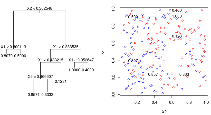
In our case, although it is true that it is probably not the best model to select to predict, it is of great interest to visualize the characteristics used to make the decisions within the decision tree. Thus, executing the decision tree model we obtain the following graph:
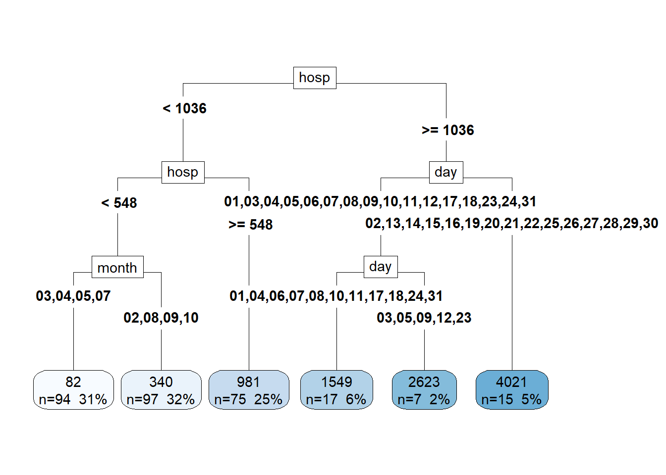 In this way, it is possible to observe the decision borders selected by the model and that are easily interpretable, which is an advantage of this model compared to other more sophisticated ones as mentioned above.
Regarding the distribution, it can be seen how clearly our model is based on decision rules to construct groups, and from there it assigns the mean of the values to all the subjects of that group. In this way, we have a total of 6 density peaks (in reference to the 6 groups) distributed in the continuous variable.
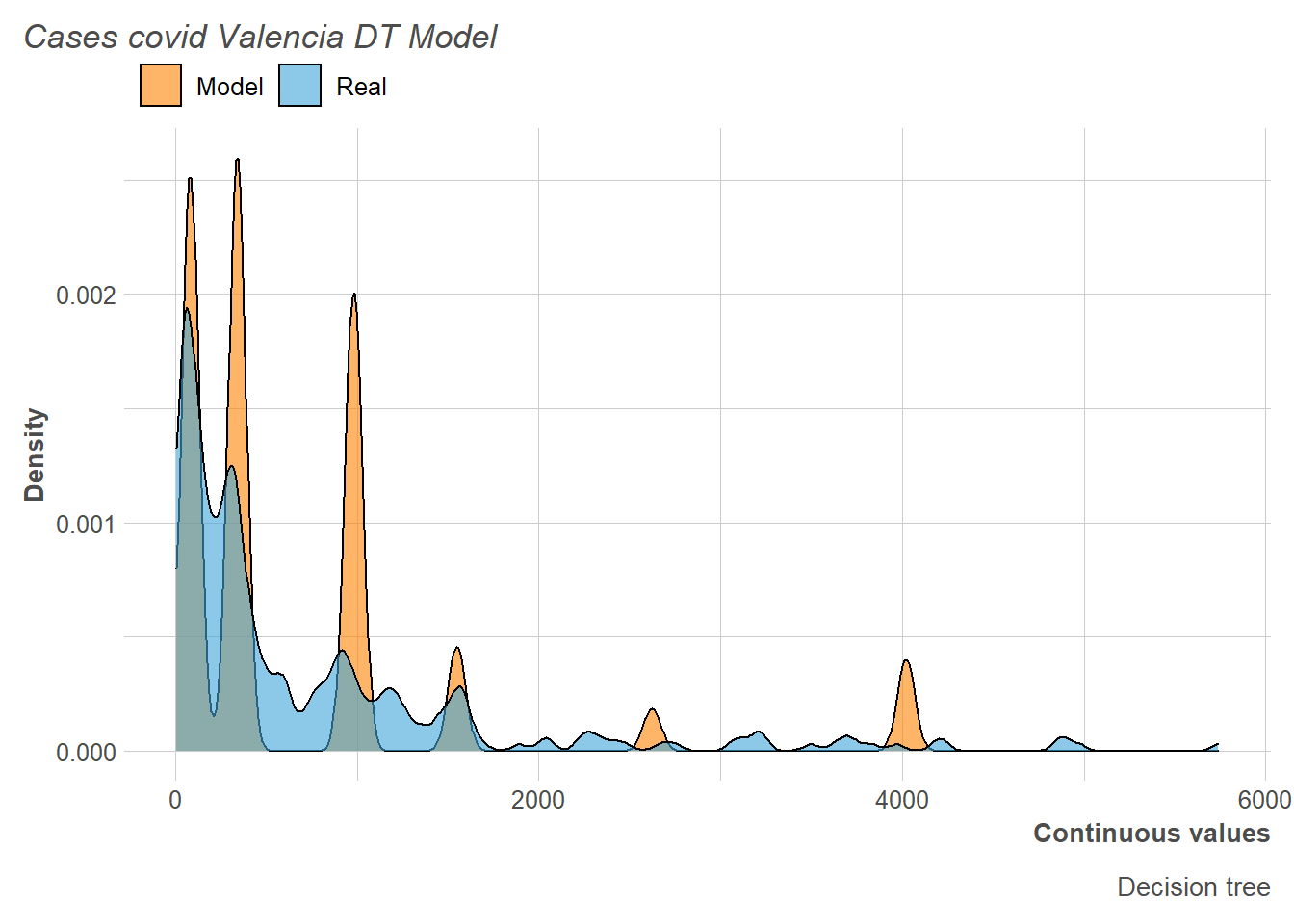
Thus, in relation to the set of tests, we observe how the values adjust them much better than the other models. This is because, precisely because it is a more regularized and simple model than those described above, it does not capture the dynamics of the distribution with the same clarity as the others, which favors it for this set of tests.
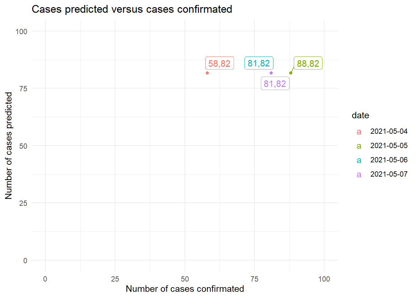 Thus, the MAE and RMSE obtained are quite good considering the test sample that we have.
| RMSE |
|---|
| 12.23997 |
| MAE |
|---|
| 7.808511 |
2.4 Random Forest (RF)
Random forest is a specific case of bootstrap aggregating, commonly known as bagging. In this way, in random forest several decision trees are trained with, usually, random training subsets of size 2/3 with respect to the total training set. Likewise, the variables to make the separations in the decision nodes are taken from a random subset of the total of variables. In this way, weak classifiers that are not highly correlated with each other are trained in parallel, which means that later, when selecting the predictive value for an instance through an average of all the trees, the variance of the model is reduced and normally good results are obtained.
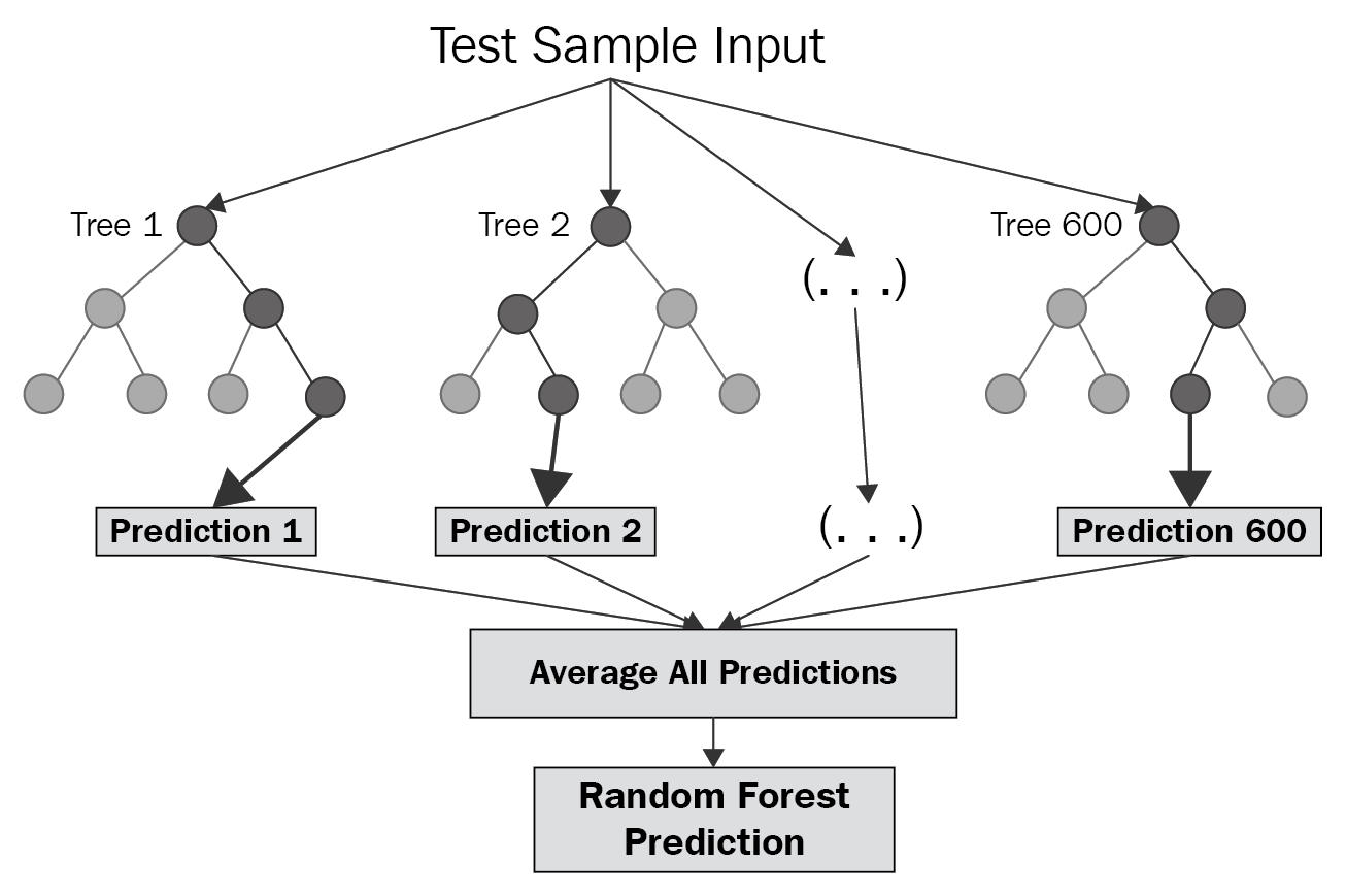
Although it is true that multiple hyperparameters can be optimized in random forests, in our case we have selected a large number of trees (500) and we have optimized the number of random characteristics that each decision node has to choose from, because it is the most relevant parameter of the RF. In this way, the results of the optimization have resulted in the random selection between 5 characteristics being optimal.
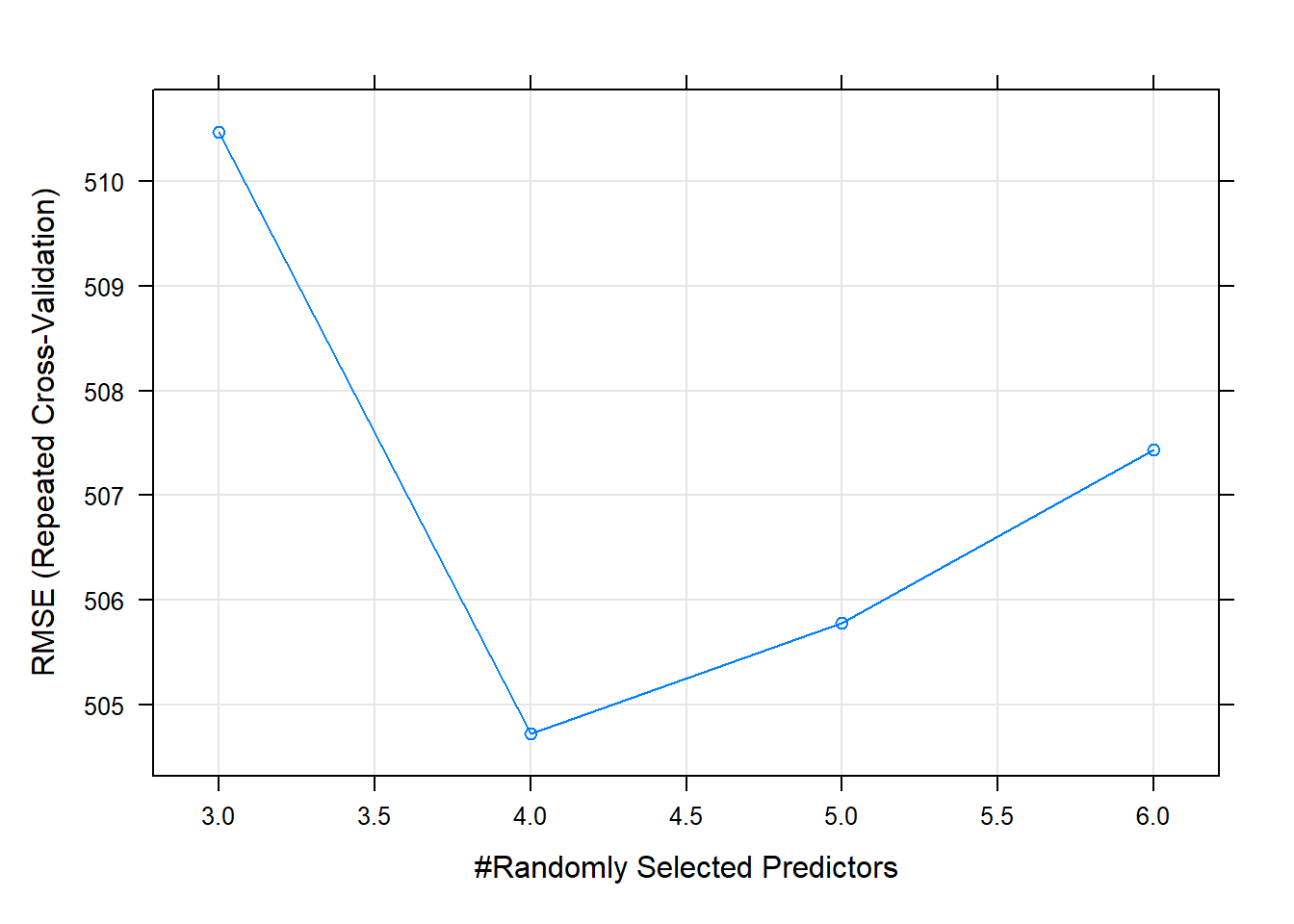
# best parameters and results of the best model
knitr::kable(get_best_result(rf_tune_v1), align = "c", "simple")| mtry | RMSE | Rsquared | MAE | RMSESD | RsquaredSD | MAESD |
|---|---|---|---|---|---|---|
| 4 | 504.7205 | 0.7595359 | 263.4705 | 77.8571 | 0.1076473 | 39.29908 |
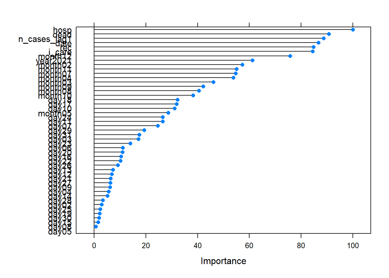
Thus, by way of illustration, we can observe in the following graph the most relevant variables selected by the RF model.
Regarding the distribution of the numbers of cases, we observed that those predicted in the training fit the real ones quite well, although a slight overestimation of the number of cases was also observed.
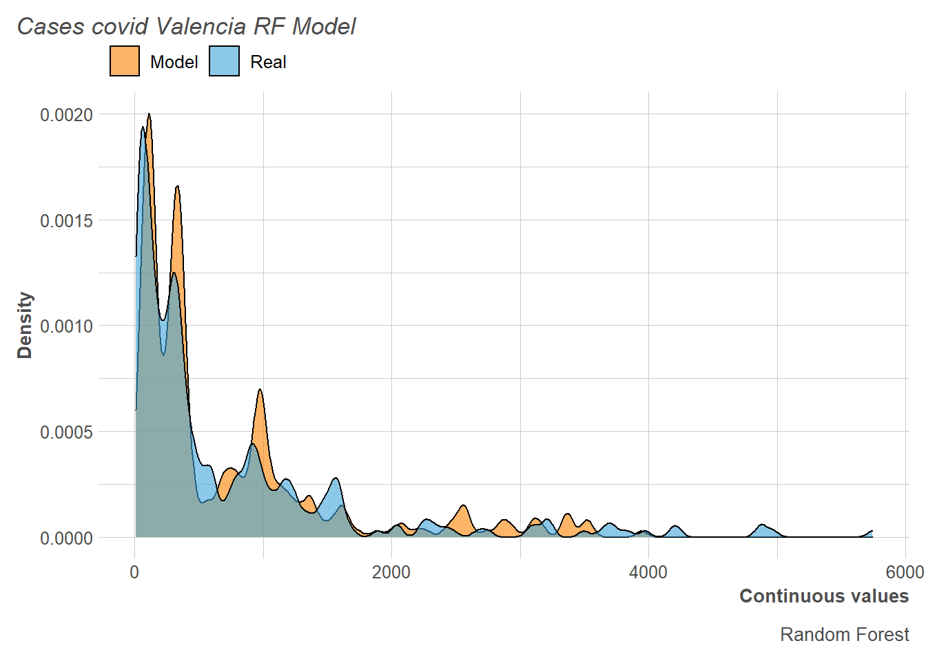
This generates that when adjusting the model with respect to the test set, the results are more or less reasonable compared to the models carried out so far.
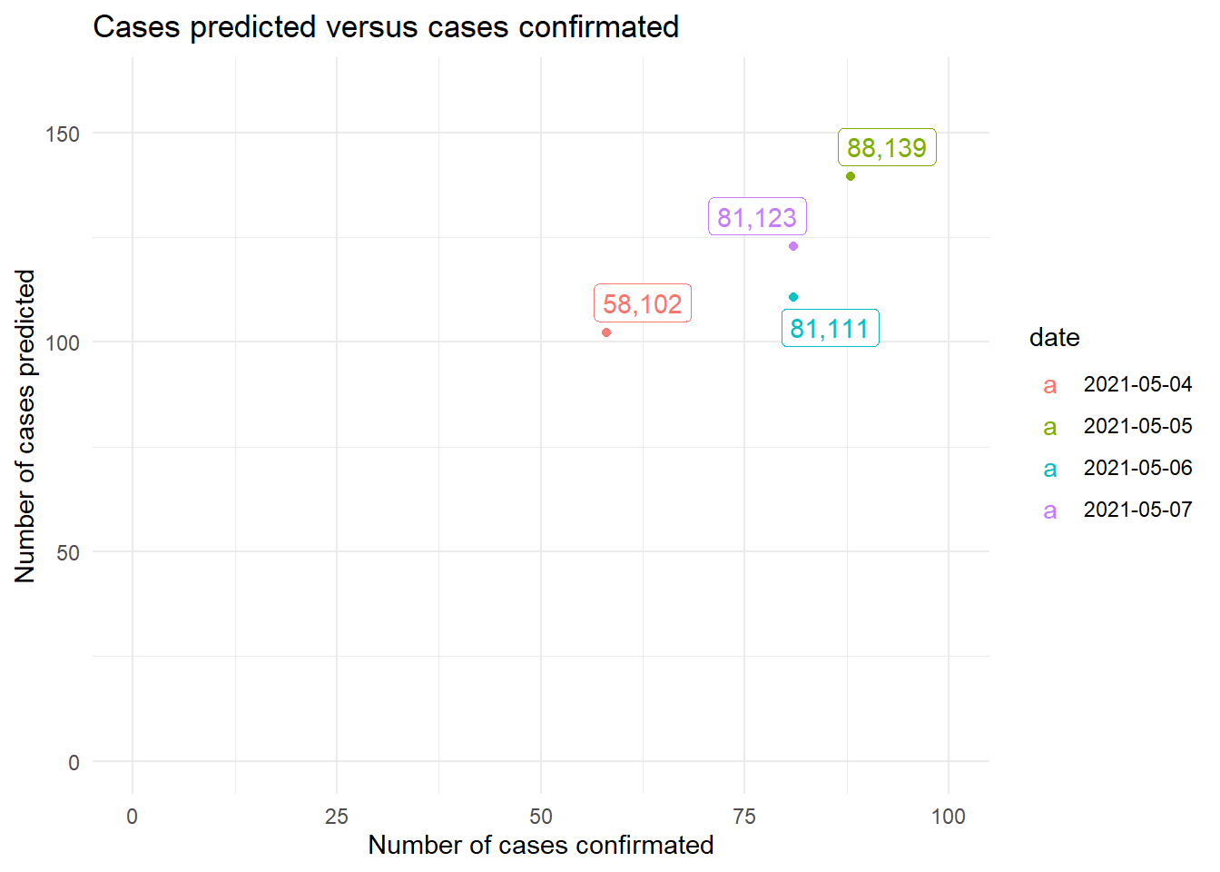
And in this way, the RMSE and the MAE obtained is quite reasonable.
| RMSE |
|---|
| 42.54705 |
| MAE |
|---|
| 41.81251 |
2.5 Extreme Grandient Boosting (XGB)
Boosting is a machine learning technique where, unlike bagging, instead of training the models in parallel, it trains multiple decision trees sequentially where the following tree is passed the weighted sample of data from the previous tree. In this way, each tree has a greater impact on the errors of the previous one, being able to obtain very good results. Although it is true that it is more prone to overfitting, it is currently one of the techniques with the best results when it comes to predicting within machine learning.
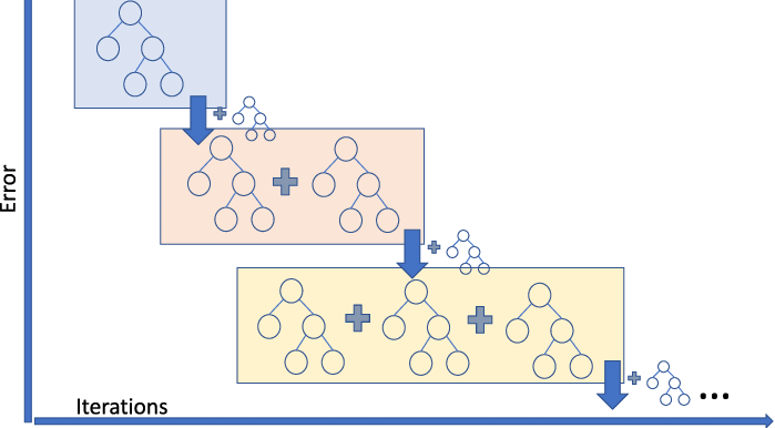
Currently, one of the models that are used the most and that give the best results is extreme gradient boosting. This consists of a boosting-type structure model that is optimized by means of a gradient and that in turn is combined with lasso, in such a way that the overfitting to which this type of models can become prone to having a low bias and a low variance.
However, they tend to be computationally expensive models since they have to optimize a large number of hyper-parameters.
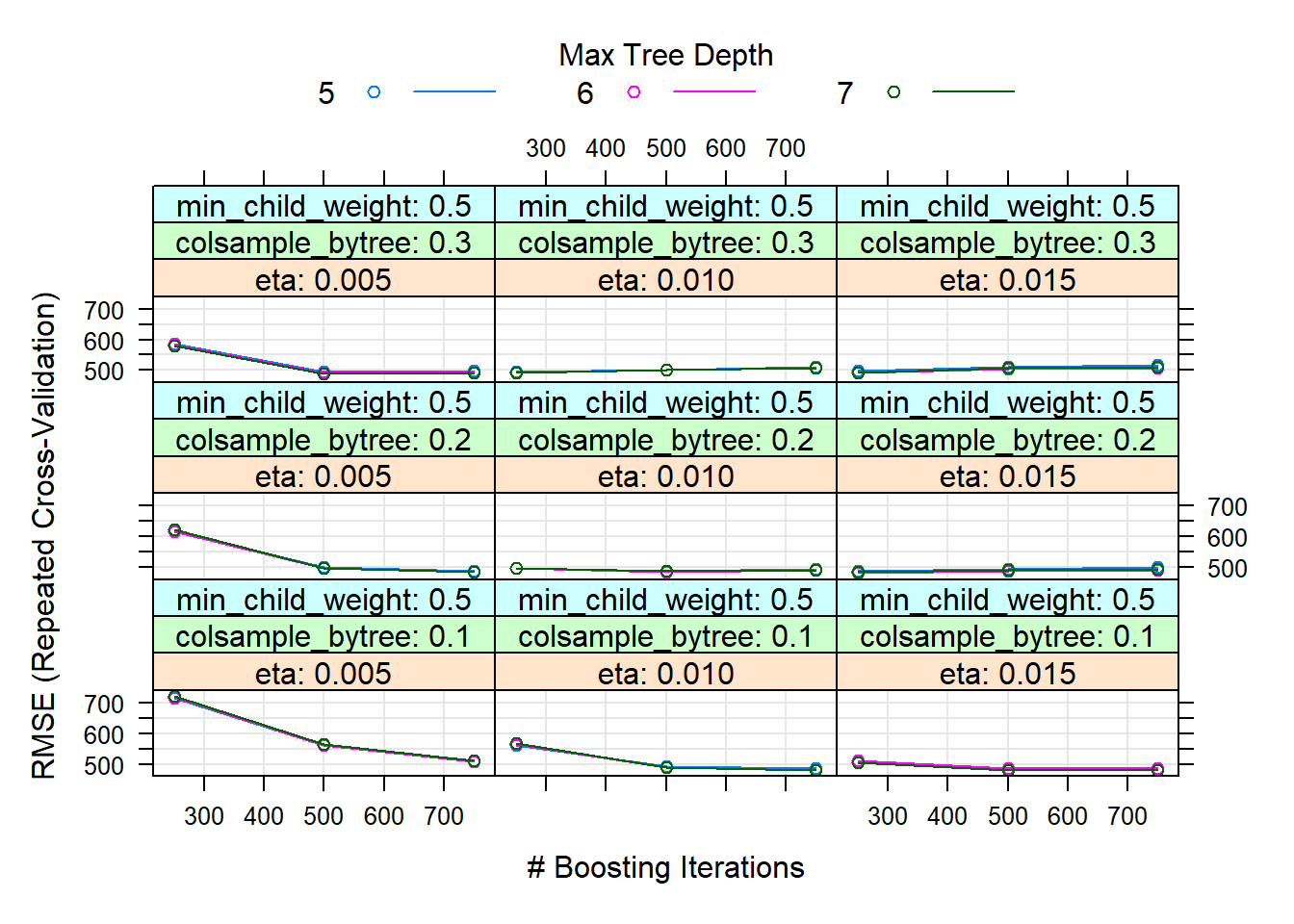
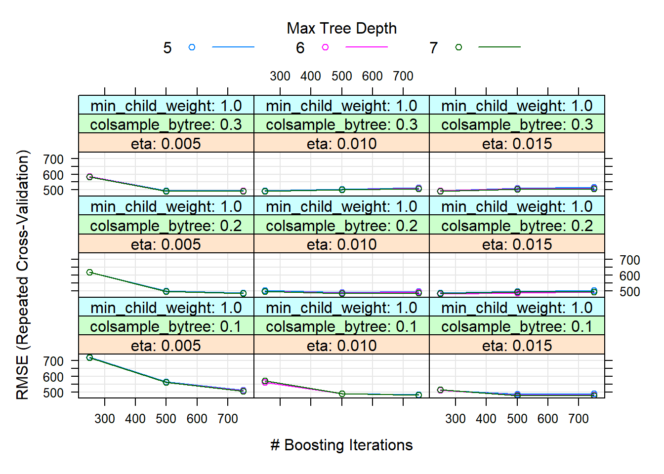
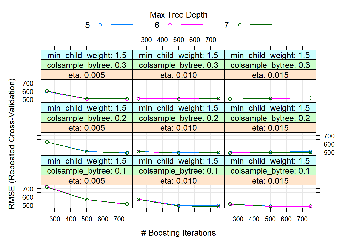
In our case, several of these have been optimized, such as the maximum depth of the trees (recommended not to be too high due to overfitting) or the weights of the instances. Thus, the best model has been with: nrounds = 500, max_depth = 7, eta = 0.015, gamma = 1, colsample_bytree = 0.1, min_child_weight = 0.5 and subsample = 1.
# best parameters and results of the best model
knitr::kable(get_best_result(xgb_tune_v1), align = "c", "simple")| eta | max_depth | gamma | colsample_bytree | min_child_weight | subsample | nrounds | RMSE | Rsquared | MAE | RMSESD | RsquaredSD | MAESD |
|---|---|---|---|---|---|---|---|---|---|---|---|---|
| 0.015 | 7 | 1 | 0.1 | 1 | 1 | 500 | 477.7426 | 0.7675768 | 252.0206 | 115.9516 | 0.1006831 | 49.48895 |
Thus, we observe that although the distribution of the number of cases predicted in the training does not fit badly, it is observed that it is clearly shifted to the right and is similar than the adjustment made by Random Forest.
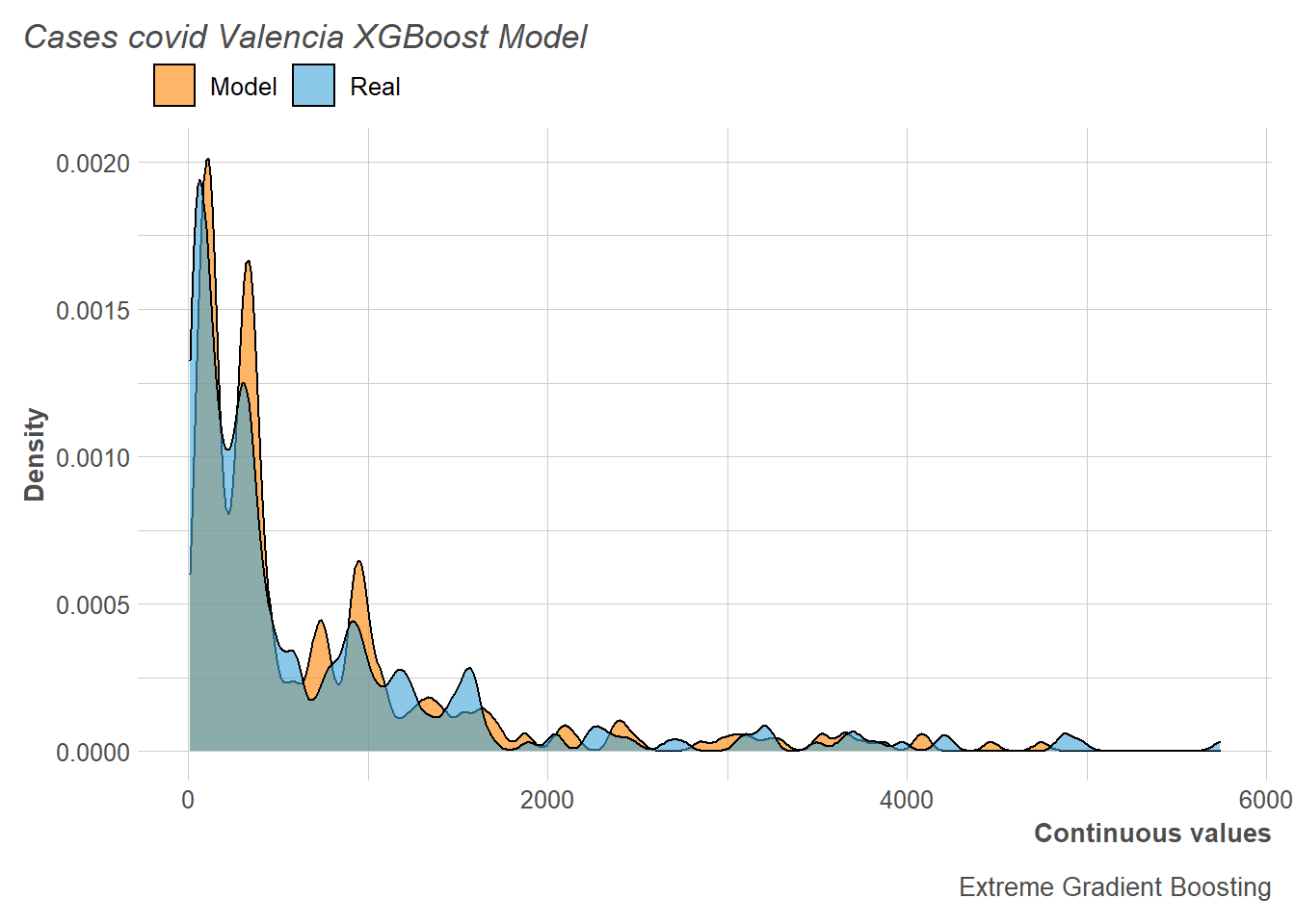
This is reflected in the predictions of the test, where it can be seen that our model overestimates the number of COVID-19 cases.
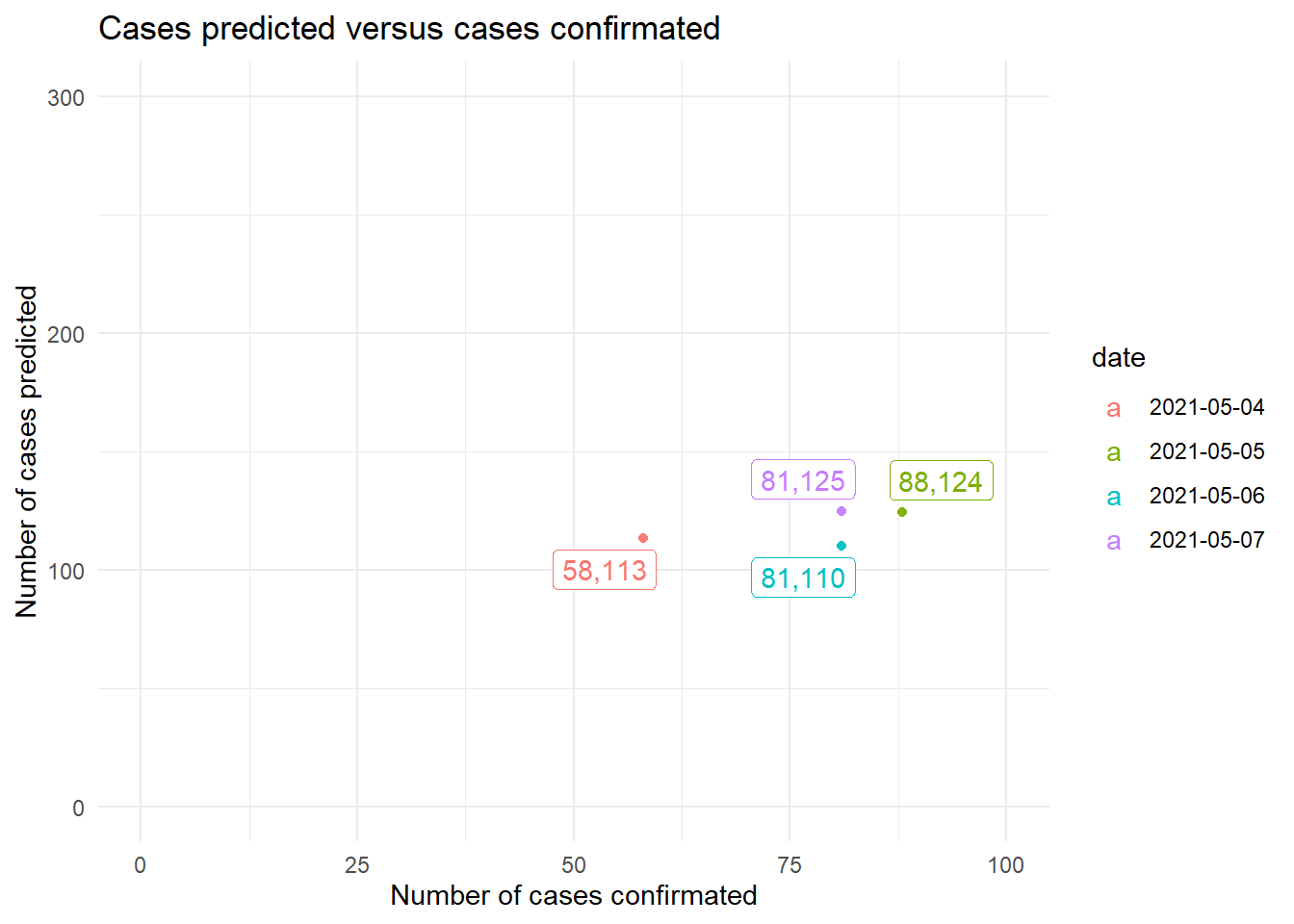
Consequently, this translates into MAE and RMSE similar than those obtained using the Random Forest.
| RMSE |
|---|
| 42.28482 |
| MAE |
|---|
| 41.15577 |
2.6 Neural Networks (NN)
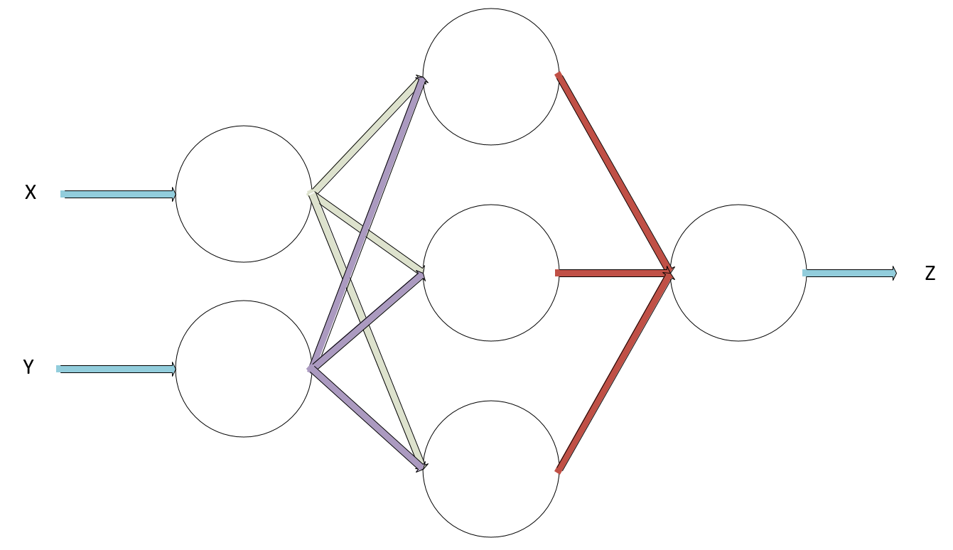
Neural networks are nothing more than a set of activation functions identical or similar to logistic regression for a set of nodes which are structured in layers. Thus, the term neural network is used when there is a total hidden layer (between the input layer and the output layer). In this way, neural networks calculate the weights of all activation functions at the same time using the descending gradient and the back-propagation algorithm. Such models, which are very popular today, tend to perform very well on very large, high-dimensional data sets.
Thus, in neuronal networks there are multiple parameters to optimize and, generally, they require a large computational expense. Also, it is usually convenient to use them in problems where other methods are not able to work as well as them.
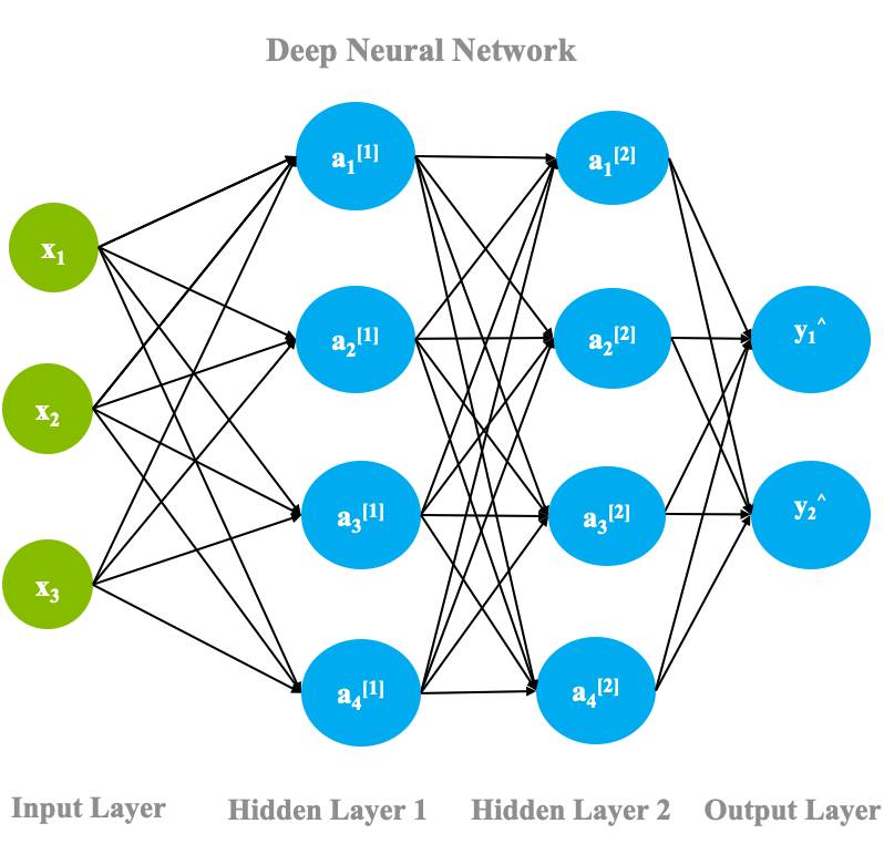
Continuing with this topic, the Deep Neural Networks (DNN) are similar to a neural network, with the difference that it has more than one hidden layer. In this way, a higher computational expense is required, with the benefit of normally obtaining better results.
Neural networks are usually quite good at predicting, however, they are black box models where we compromise the interpretability of the model in order to obtain good predictions.
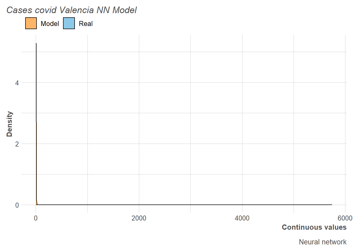
Regarding the adjustment made for the simple neural networks, it should be noted that it has not been possible to make it work properly, since one of the main complications of this type of method is that it is necessary to have experience building network architectures so that it does not happen. what is presented in this situation. Thus, we observe very high values of RMSE and MAE of the training set that we will see as it affects the estimation of the distribution of the number of cases.

# best parameters and results of the best model
knitr::kable(get_best_result(nn_tune_v1), align = "c", "simple")| size | decay | RMSE | Rsquared | MAE | RMSESD | RsquaredSD | MAESD |
|---|---|---|---|---|---|---|---|
| 1 | 0.005 | 1199.293 | NaN | 717.5694 | 167.9535 | NA | 67.24493 |
Thus, it can be seen how the network has not learned anything and places all the predictions in a value, generating the practically imperceptible distribution that we observe.
The same network architecture problem has been experienced with the deep neural network, where it becomes even more important to have knowledge of initial architectures on which to improve. Also, another possibility to find a good architecture is to have GPUs with which to run many possible variants of layers and neurons. However, this possibility requires considerable time and resource consumption. On the other hand, we also have little data, which is a very important aggravating factor in prediction using neural networks.
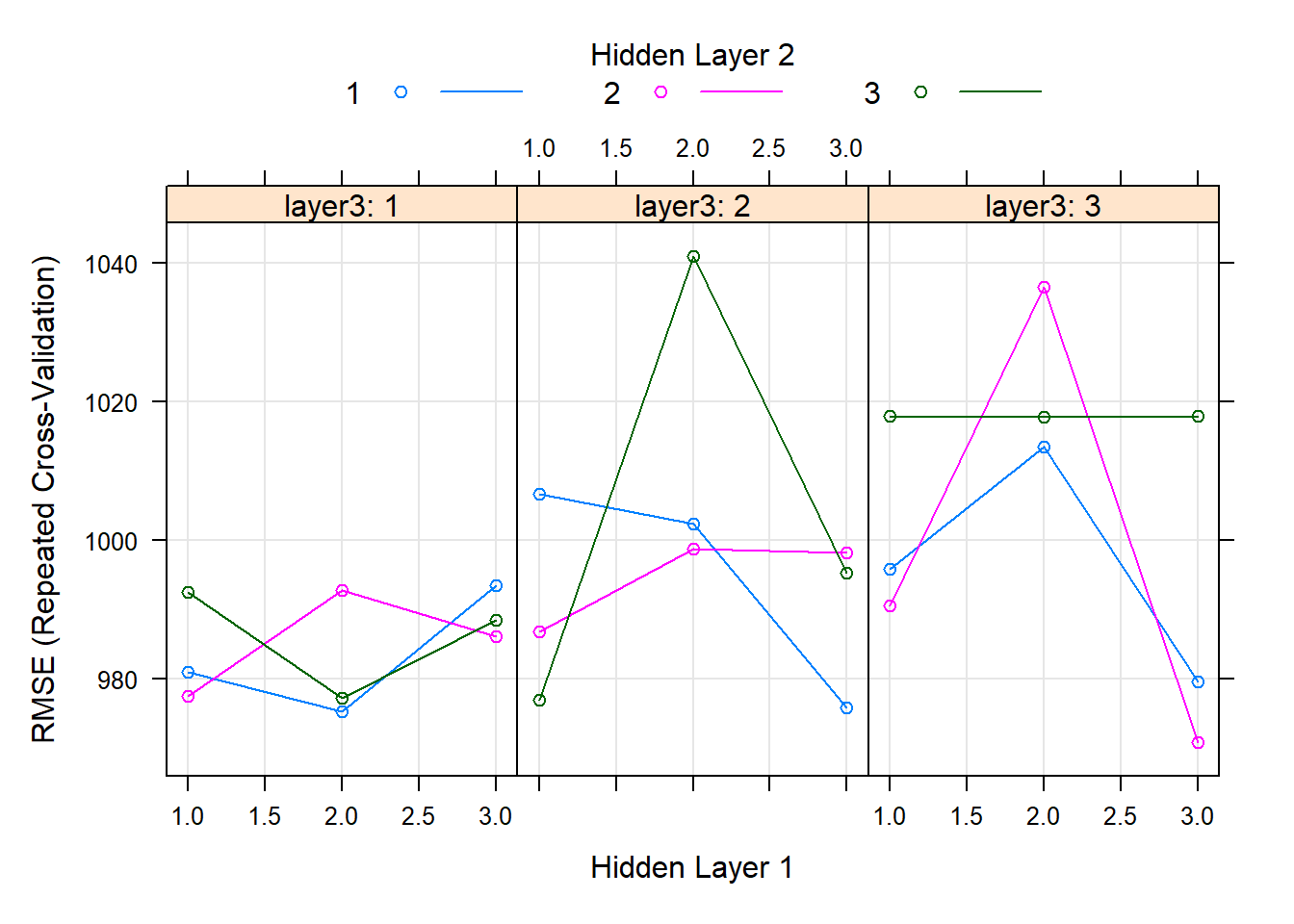
# best parameters and results of the best model
knitr::kable(get_best_result(dnn_tune_v0), align = "c", "simple")| layer1 | layer2 | layer3 | hidden_dropout | visible_dropout | RMSE | Rsquared | MAE | RMSESD | RsquaredSD | MAESD |
|---|---|---|---|---|---|---|---|---|---|---|
| 3 | 2 | 3 | 0 | 0 | 970.8477 | 0.2886199 | 652.6269 | 141.9388 | 0.1246105 | 87.07022 |
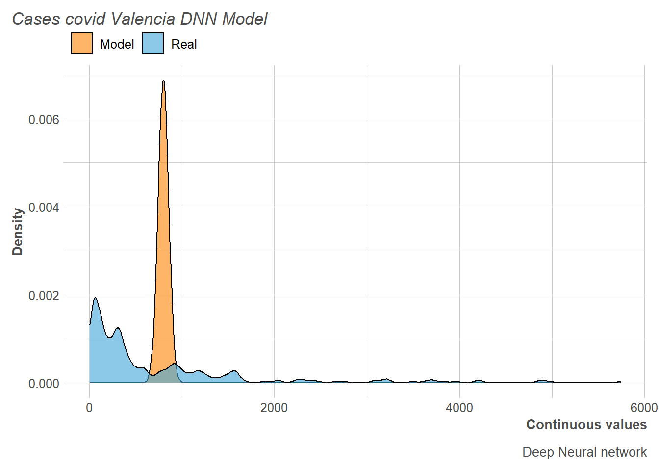
In this way, it can be seen how the neural network is not capable of capturing the trend of the training data and locates all its predictions in a single point.
2.7 Ensemble of Models
Ensembles are sets of models, which are combined to obtain better and more robust predictions. In this way, it is usually used with the best models, and it is preferable that these models are not correlated because otherwise the gain we have when using an ensemble is very low. However, even if we do not gain more predictive capacity, and even if we lose a little, it is still the best model when it comes to predicting future instances.
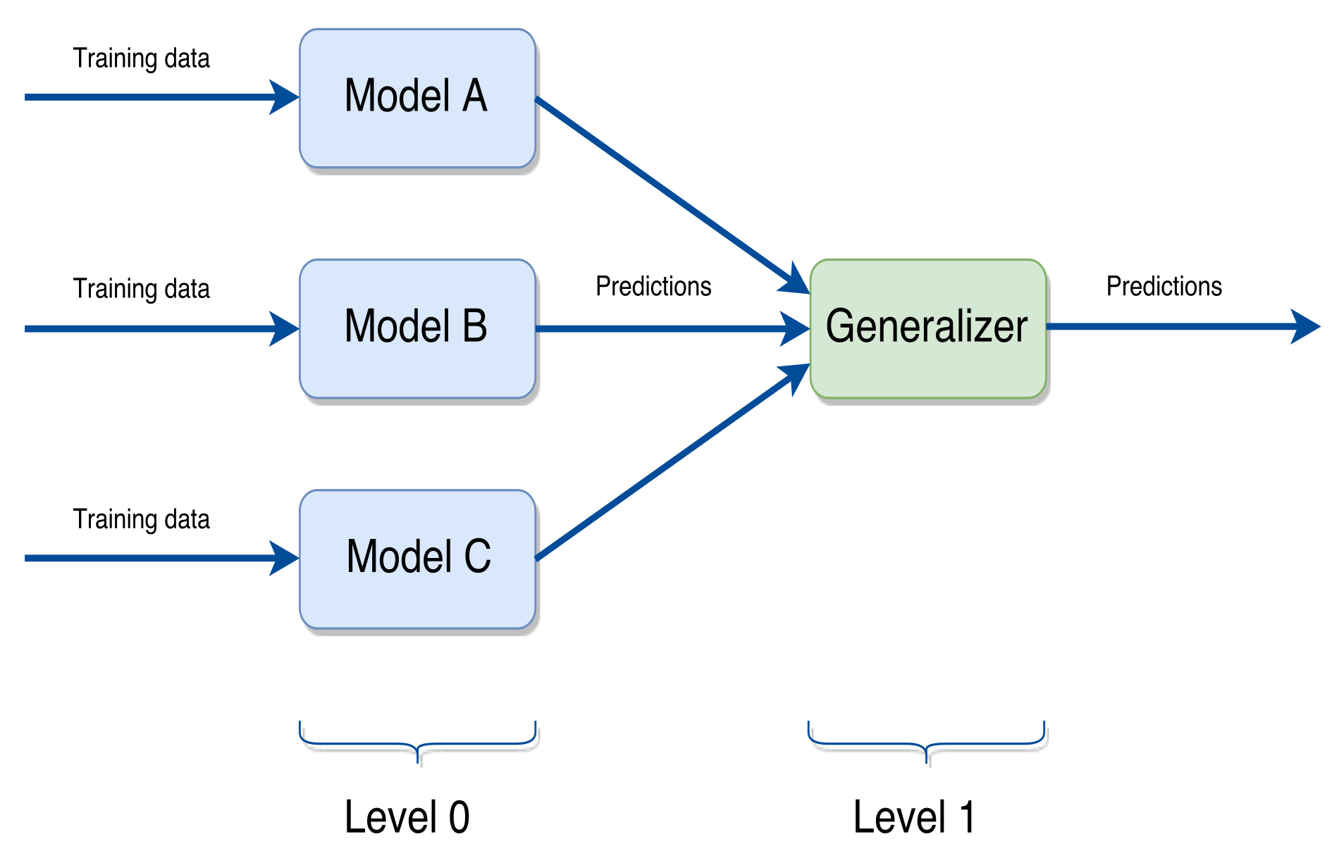
To make the ensemble of models, the stack method has been used. In this method, basically what is done is to make the predictions of several models enter another model and this is the one that of the final predictions, improving the results obtained by being able to use the variability and results of the previous models. In our case, we have opted to introduce all the models used except the neural networks (since their prediction has not been correct), and then carry out the stacking using a random forest, since it has been observed that of the models tested it is of the best.
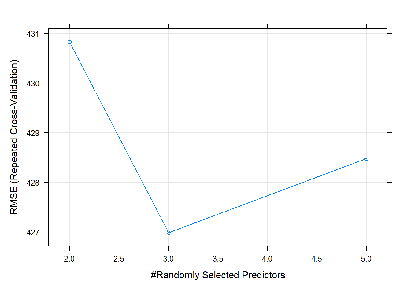
Thus, the number of optimal input variables selected by the stacking Random Forest has been equal to 3.
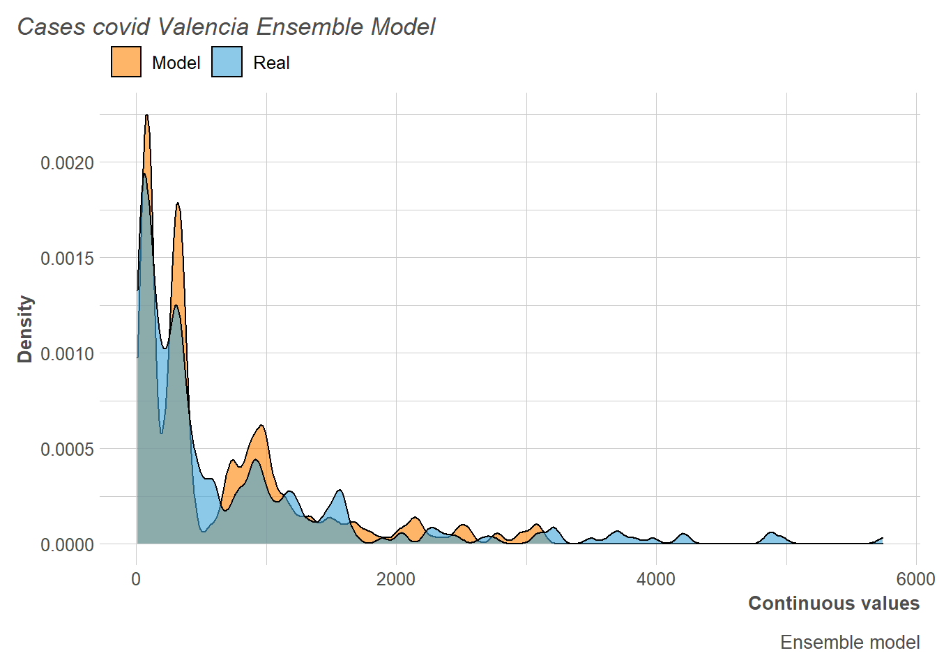
Likewise, if we look at the distribution of new COVID-19 cases daily for the training set, we can see how the distribution predicts quite well.
Consequently, this is reflected in the estimates of the test set as we can see.
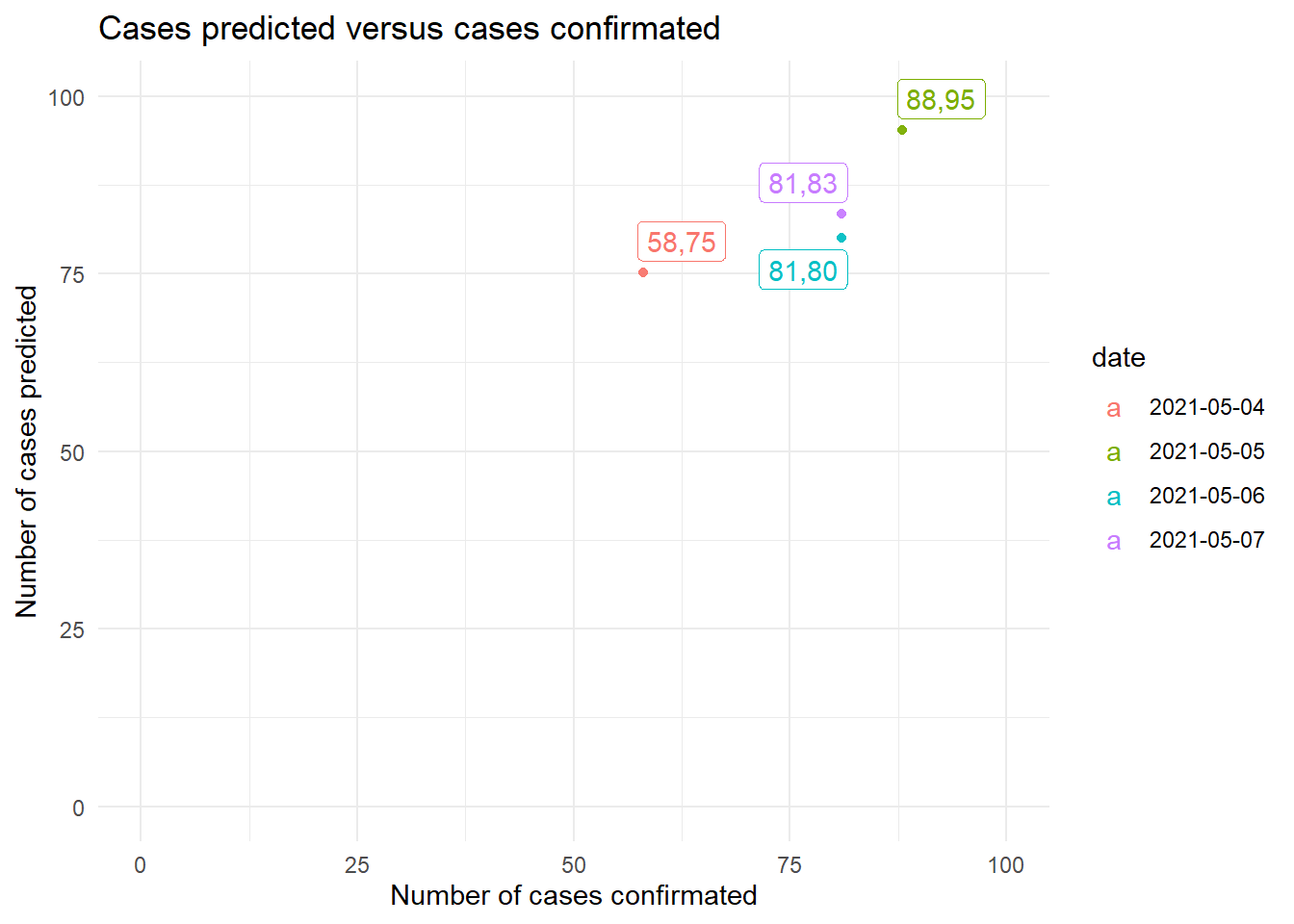
And likewise, this translates into having the best RMSE and MAE metrics of all the models. This makes sense since, although the ensemble’s interpretability is practically impossible, combining several models allows us to find a really good prediction. taking into account the little data we have, which is daily and that the test set is nothing like the train set.
| RMSE |
|---|
| 9.375921 |
| MAE |
|---|
| 6.905033 |