Chapter 2 Basic Quantities and Models

Let $X$ be a nonnegative characterize variable from a homogeneous populaton. There are five functions characterize the distribution of $X$, say:

• survival function $S(x)$
• hazard rate/risk function $h(x)$
• probability density function $f(x)$
• mean residual life at time $x$ $mrl(x)$
• cumulative hazard function $H(x)$

Survival function

The probability of an individual surviving beyond time $x$ is defined as $$\begin{equation} S(x) = Pr(X > x) = 1- F(x) = \int_x^\infty f(t)dt \tag{2.1} \end{equation}$$

where $S(x)$ is referred to as the survival function or reliability function.

Therefore based on (2.1),

$$f(x) = -\frac{dS(x)}{dx}$$ For discrete case $$S(x) = Pr(X > x) = \sum_{x_j > x} p(x_j)$$ where $p(x_j) = Pr(X = x_j)$ is the pmf.

Example for Weibull distribution

$$S(x) = \exp(-\lambda x^\alpha)$$ When $\alpha = 1$, it becomes exponential distribution.

f1 <- function(x) exp(-0.26328 * x^0.5)
f2 <- function(x) exp(-0.1 * x)
f3 <- function(x) exp(-0.00208 * x^3)
curve(f1, from = 0, to = 20, ylim = c(0, 1), ylab = "Survival Prob")
curve(f2, from = 0, to = 20, add = T, col = "red")
curve(f3, from = 0, to = 20, add = T, col = "blue")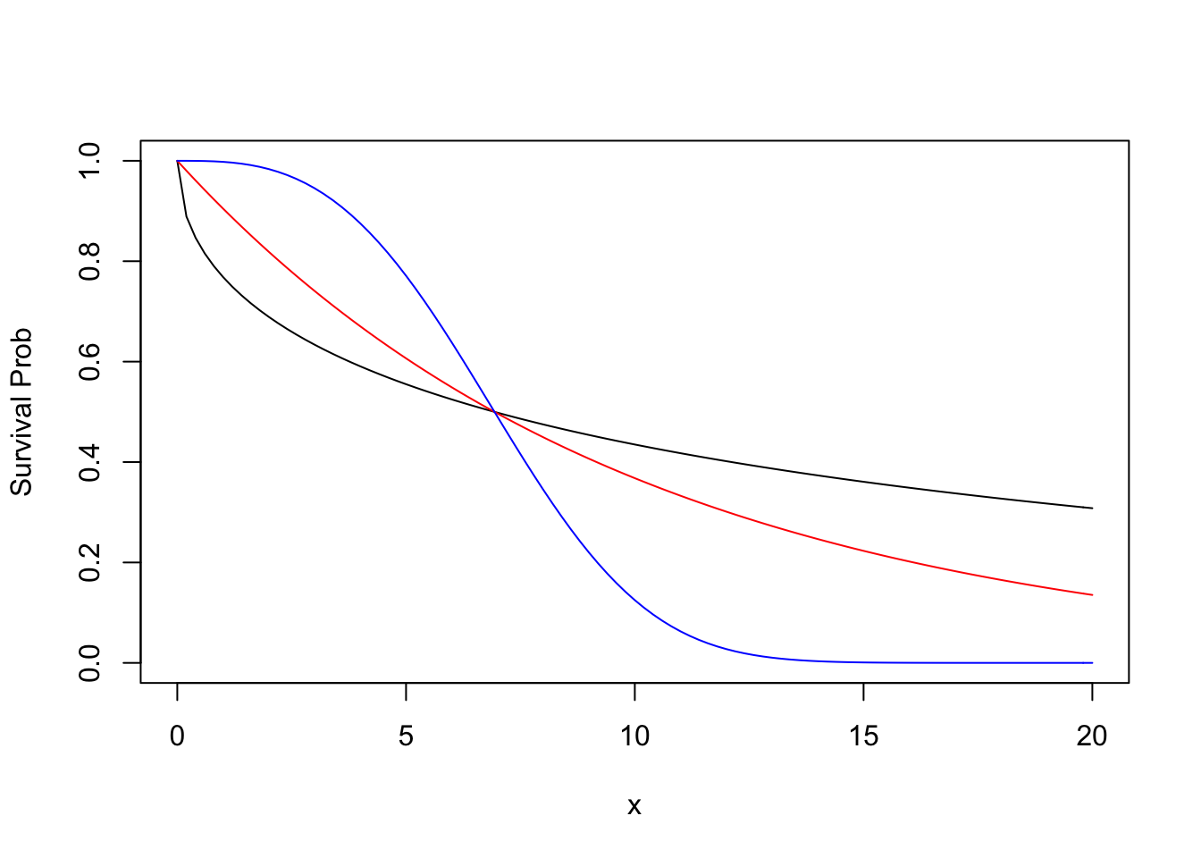

Hazard Function

Hazard function is also known as the conditional failure rate in reliability, the force of mortality in demography, the intensity function in stochastic processes, the age-specific failure rate in epidemiology, the inverse of the Mill’s ratio in economics, or simply as the hazard rate.

$$h(x)=\lim _{\Delta x \rightarrow 0} \frac{P[x \leq X<x+\Delta x \mid X \geq x]}{\Delta x} \tag{2.2}$$ From (2.2), $h(x)dx$ can be viewed as the “approximate” probability of an individual of age $x$ experiencing the event in the next instant.

If $X$ is continuous, then $$h(x) = f(x)/S(x) = -\frac{d\ln S(x)}{dx} \tag{2.3}$$ In other word, $$S(x) = \exp[-H(x)] = \exp[-\int_0^x h(u)du] \tag{2.4}$$ When $X$ is discrete, $$h\left(x_j\right)=\operatorname{Pr}\left(X=x_j \mid X \geq x_j\right)=\frac{p\left(x_j\right)}{S\left(x_{j-1}\right)} = 1 - \frac{S\left(x_{j}\right)}{S\left(x_{j-1}\right)}, \quad j=1,2, \ldots$$ The survival function can be written as the product of conditional survival probabilities: $$S(x) = \prod_{x_j \leq x}S(x_j)/S(x_{j-1}) = \prod_{x_j \leq x}[1-h(x_j)]$$

Example for Weibull distribution

For Weibull distribution, the hazard function is $$h(x) = \alpha\lambda x^{\alpha - 1}$$

curve(0.26328 * 0.5 * x^-0.5, from = 0, to = 10, ylim = c(0, 1), ylab = "Hazard Rate")
curve(0.1*x^0, from = 0, to = 20, add = T, col = "red")
curve(0.00208 * 3 * x^2, from = 0, to = 20, add = T, col = "blue")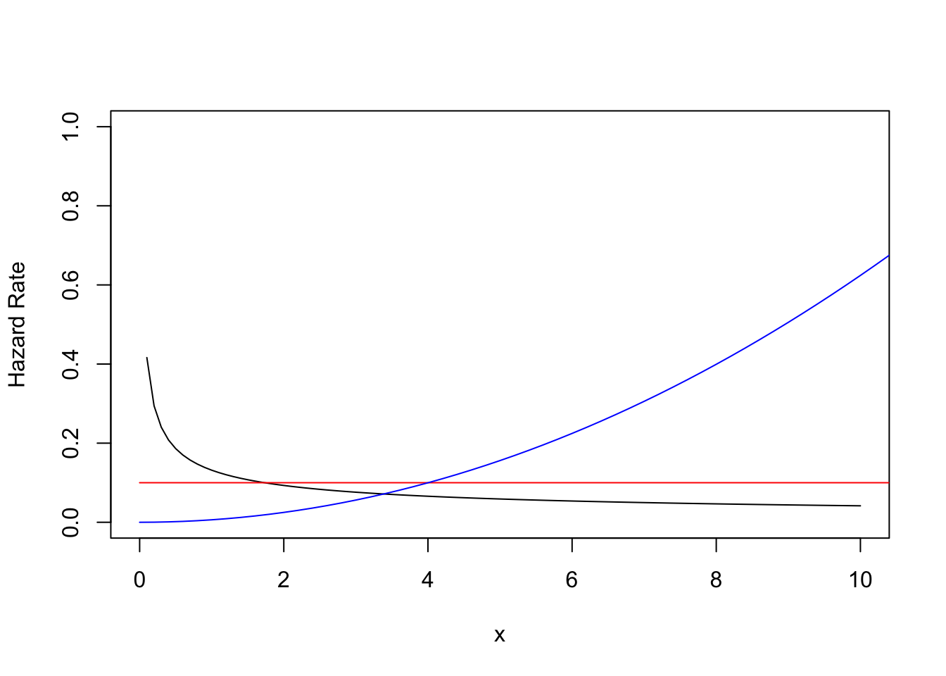

Cumulative hazard function

$$H(x) = \int_0^x h(u)du = -\ln S(x) \tag{2.5}$$ For discrete $X$, $$H(x) = \sum_{x_j \leq x} h(x_j)$$ When $X$ is discrete, $S(x) = \exp[-H(x)]$ is no longer holds for true.

Mean residual life function and median life

The parameter measures the expected remaining lifetime $mrl(x)$ is defined as

$$mrl(x) = E(X - x\mid X > x) = \frac{\int_x^\infty (t - x)f(t)dt}{S(x)} = \frac{\int_x^\infty S(t)dt}{S(x)} \tag{2.6}$$

Note:

$$\mu = E(X) = \int_0^\infty tf(t) dt = \int_0^\infty S(t) dt$$ $$Var(X) = 2 \int_0^\infty tS(t) dt - [ \int_0^\infty S(t)dt]^2$$

Examples:

• The mean and median lifetimes for an exponential life distribution are $1/\lambda$ and $(\ln 2)/\lambda$.
• The $100p$th percentile for the Weibull distribution is found by solving $1 - p = \exp\{-\lambda x_p^\alpha\}$ so $x_p = \{-\ln [1-p]/\lambda \}^{1/\alpha}$

Common parametric models

Distribution	$f(x)$	$S(x)$	$h(x)$	$E(X)$
Exponential	$\lambda\exp(-\lambda x)$	$\exp[-\lambda x]$	$\lambda$	$1/\lambda$
Weibull	$\alpha\lambda x^{\alpha - 1}\exp(-\lambda x^\alpha)$	$\exp[-\lambda x^\alpha]$	$\alpha\lambda x^{-\alpha - 1}$	$\frac{\Gamma(1 + 1/\alpha)}{\lambda^{1/\alpha}}$
Gamma	$\frac{\lambda^\beta x^{\beta - 1} \exp(-\lambda x)}{\Gamma(\beta)}$	$1 - I(\lambda x, \beta)^*$	$\frac{f(x)}{S(x)}$	$\beta/\lambda$
Log normal	$\frac{\exp \left[-\frac{1}{2}\left(\frac{\ln x-\mu}{\sigma}\right)^2\right]}{x(2 \pi)^{1 / 2} \sigma}$	$1 - \Phi(\frac{\ln x - \mu}{\sigma})$	$\frac{f(x)}{S(x)}$	$\exp(\mu + 0.5\sigma^2)$
Log logistic	$\frac{\alpha x^{\alpha - 1} \lambda}{[1 + \lambda x^\alpha]^2}$	$\frac{1}{1 + \lambda x^\alpha}$	$\frac{\alpha x^{\alpha - 1}\lambda}{1 + \lambda x^\alpha}$	$\frac{\pi \operatorname{Csc}(\pi / \alpha)}{\alpha \lambda^{1 / \alpha}} \text { if } \alpha>1$
Gompertz	$\theta e^{\alpha x} \exp [\frac{\theta}{\alpha}(1-e^{\alpha x})]$	$\exp[\frac{\theta}{\alpha}(1-e^{\alpha x})]$	$\theta e^{\alpha x}$	$\int_0^\infty S(x) dx$
Pareto	$\frac{\theta \lambda^\theta}{x^{\theta + 1}}$	$\frac{\lambda^\theta}{x^\theta}$	$\frac{\theta}{x}$	$\frac{\theta\lambda}{\theta - 1}$ if $\theta > 1$

where $I(t, \beta) = \int_0^t u^{\beta - 1} \exp(-u) du/\Gamma(\beta)$