Chapter 5 Analysis of Covariance (ANCOVA)

library(tidyverse)  # ggplot2, tidyr, dplyr
library(emmeans)

5.1 Introduction

One way that we could extend the ANOVA and regression models is to have both categorical and continuous predictor variables. For historical reasons going back to pre “computer in your pocket” days, statisticians call this the Analysis of Covariance (ANCOVA) model. Because it is just another example of a \(\boldsymbol{y} = \boldsymbol{X\beta} + \boldsymbol{\epsilon}\) linear model, I prefer to think of it as simply having both continuous and categorical variables in my model. None of the cookbook calculations change, but the interpretation of the parameters gets much more interesting.

The dataset teengamb in the package faraway has data regarding the rates of gambling among teenagers in Britain and their gender and socioeconomic status. One question we might be interested in is how gender and income relate to how much a person gambles. But what should be the effect of gender be?

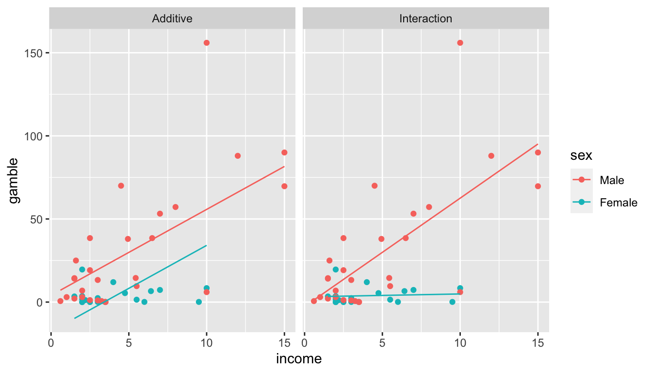
There are two possible ways that gender could enter the model. Either:

We could fit two lines to the data one for males and one for females but require that the lines be parallel (i.e. having the same slopes for income). This is accomplished by having a separate y-intercept for each gender. In effect, the line for the females would be offset by a constant amount from the male line.
We could fit two lines but but allow the slopes to differ as well as the y-intercept. This is referred to as an “interaction” between income and gender. One way to remember that this is an interaction is because the effect of income on gambling rate is dependent on the gender of the individual.

*It should be noted here, that the constant variance assumption is being violated and we really ought to do a transformation. I would recommend performing a \(\sqrt{\cdot}\) transformation on both the gamble and income covariates, but we’ll leave them as is for now.

We will now see how to go about fitting these two models. As might be imagined, these can be fit in the same fashion we have been solving the linear models, but require a little finesse in defining the appropriate design matrix \(\boldsymbol{X}\).

5.2 Offset parallel Lines (aka additive models)

In order to get offset parallel lines, we want to write a model \[y_{i}=\begin{cases} \beta_{0}+\beta_{1}+\beta_{2}x_{i}+\epsilon_{i} & \;\;\;\textrm{if female}\\ \beta_{0}+\beta_{2}x_{i}+\epsilon_{i} & \;\;\;\textrm{if male} \end{cases}\] where \(\beta_{1}\) is the vertical offset of the female group regression line to the reference group, which is the males regression line. Because the first \(19\) observations are female, we can this in in matrix form as \[\left[\begin{array}{c} y_{1}\\ \vdots\\ y_{19}\\ y_{20}\\ \vdots\\ y_{47} \end{array}\right]=\left[\begin{array}{ccc} 1 & 1 & x_{1}\\ \vdots & \vdots & \vdots\\ 1 & 1 & x_{19}\\ 1 & 0 & x_{20}\\ \vdots & \vdots & \vdots\\ 1 & 0 & x_{47} \end{array}\right]\left[\begin{array}{c} \beta_{0}\\ \beta_{1}\\ \beta_{2} \end{array}\right]+\left[\begin{array}{c} \epsilon_{1}\\ \vdots\\ \epsilon_{19}\\ \epsilon_{20}\\ \vdots\\ \epsilon_{47} \end{array}\right]\]

I like this representation where \(\beta_{1}\) is the offset from the male regression line because it makes it very convenient to test if the offset is equal to zero. The second column of the design matrix referred to as a “dummy variable” or “indicator variable” that codes for the female gender. Notice that even though I have two genders, I only had to add one additional variable to my model because we already had a y-intercept \(\beta_{0}\) and we only added one indicator variable for females.

What if we had a third group? Then we would fit another column of indicator variable for the third group. The new beta coefficient in the model would be the offset of the new group to the reference group. For example we consider \(n=9\) observations with \(n_i=3\) observations per group where \(y_{i,j}\)is the \(j\) th replication of the \(i\)th group. \[\left[\begin{array}{c} y_{1,1}\\ y_{1,2}\\ y_{1,3}\\ y_{2,1}\\ y_{2,2}\\ y_{2,3}\\ y_{3,1}\\ y_{3,2}\\ y_{3,3} \end{array}\right]=\left[\begin{array}{cccc} 1 & 0 & 0 & x_{1,1}\\ 1 & 0 & 0 & x_{1,2}\\ 1 & 0 & 0 & x_{1,3}\\ 1 & 1 & 0 & x_{2,1}\\ 1 & 1 & 0 & x_{2,2}\\ 1 & 1 & 0 & x_{2,3}\\ 1 & 0 & 1 & x_{3,1}\\ 1 & 0 & 1 & x_{3,2}\\ 1 & 0 & 1 & x_{3,3} \end{array}\right]\left[\begin{array}{c} \beta_{0}\\ \beta_{1}\\ \beta_{2}\\ \beta_{3} \end{array}\right]+\left[\begin{array}{c} \epsilon_{1,1}\\ \epsilon_{1,2}\\ \epsilon_{1,3}\\ \epsilon_{2,1}\\ \epsilon_{2,2}\\ \epsilon_{2,3}\\ \epsilon_{3,3}\\ \epsilon_{3,2}\\ \epsilon_{3,3} \end{array}\right] \]

In this model, \(\beta_0\) is the y-intercept for group \(1\). The parameter \(\beta_1\) is the vertical offset from the reference group (group \(1\)) for the second group. Similarly \(\beta_2\) is the vertical offset for group \(3\). All groups will share the same slope, \(\beta_4\).

5.3 Lines with different slopes (aka Interaction model)

We can now include a discrete random variable and create regression lines that are parallel, but often that is inappropriate, such as in the teenage gambling dataset. We want to be able to fit a model that has different slopes. \[y_{i}=\begin{cases} \left(\beta_{0}+\beta_{1}\right)+\left(\beta_{2}+\beta_{3}\right)x_{i}+\epsilon_{i} & \;\;\;\textrm{if female}\\ \beta_{0}+\beta_{2}x_{i}+\epsilon_{i} & \;\;\;\textrm{if male} \end{cases} \] Where \(\beta_{1}\) is the offset in y-intercept of the female group from the male group, and \(\beta_{3}\) is the offset in slope. Now our matrix formula looks like

\[\left[\begin{array}{c} y_{1}\\ \vdots\\ y_{19}\\ y_{20}\\ \vdots\\ y_{47} \end{array}\right]=\left[\begin{array}{cccc} 1 & 1 & x_{1} & x_{1}\\ \vdots & \vdots & \vdots & \vdots\\ 1 & 1 & x_{19} & x_{19}\\ 1 & 0 & x_{20} & 0\\ \vdots & \vdots & \vdots & \vdots\\ 1 & 0 & x_{47} & 0 \end{array}\right]\left[\begin{array}{c} \beta_{0}\\ \beta_{1}\\ \beta_{2}\\ \beta_{3} \end{array}\right]+\left[\begin{array}{c} \epsilon_{1}\\ \vdots\\ \epsilon_{19}\\ \epsilon_{20}\\ \vdots\\ \epsilon_{47} \end{array}\right] \]

where the new fourth column is the what I would get if I multiplied the \(\boldsymbol{x}\) column element-wise with the dummy-variable column. To fit this model in R we have

data('teengamb', package='faraway')

# Forces R to recognize that 0, 1 are categorical, also
# relabels the levels to something I understand.
teengamb <- teengamb %>% mutate( sex = ifelse( sex==1, 'Female', 'Male') )

# Fit a linear model with the interaction of sex and income
# Interactions can be specified useing a colon :
m1 <- lm( gamble ~ 1 + sex + income + sex:income, data=teengamb )  
m1 <- lm( gamble ~     sex + income + sex:income, data=teengamb )  

# R allows a shortcut for the prior definition
m1 <- lm( gamble ~ sex * income, data=teengamb )

# save the fit, lwr, upr values for each observation
# these are the yhat and CI 
# If columns for fit, upr, lwr are already present, remove them
teengamb <- teengamb %>%
  dplyr::select( -matches('fit'), -matches('lwr'), -matches('upr') ) %>%
  cbind( predict(m1, interval='conf') )

# Make a nice plot that includes the regression line.
ggplot(teengamb, aes(x=income, col=sex, fill=sex)) + 
      geom_ribbon(aes(ymin=lwr, ymax=upr),
                  alpha=.3) +   # how solid the layer is
      geom_point(aes(y=gamble)) +
      geom_line(aes(y=fit))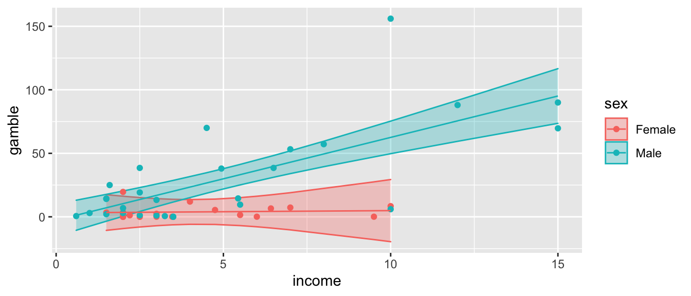

# print the model summary
summary(m1)

## 
## Call:
## lm(formula = gamble ~ sex * income, data = teengamb)
## 
## Residuals:
##     Min      1Q  Median      3Q     Max 
## -56.522  -4.860  -1.790   6.273  93.478 
## 
## Coefficients:
##                Estimate Std. Error t value Pr(>|t|)   
## (Intercept)      3.1400     9.2492   0.339  0.73590   
## sexMale         -5.7996    11.2003  -0.518  0.60724   
## income           0.1749     1.9034   0.092  0.92721   
## sexMale:income   6.3432     2.1446   2.958  0.00502 **
## ---
## Signif. codes:  0 '***' 0.001 '**' 0.01 '*' 0.05 '.' 0.1 ' ' 1
## 
## Residual standard error: 20.98 on 43 degrees of freedom
## Multiple R-squared:  0.5857, Adjusted R-squared:  0.5568 
## F-statistic: 20.26 on 3 and 43 DF,  p-value: 2.451e-08

To interpret the terms, we have

Coefficients	Interpretation
`(Intercept)`	y-intercept for the females
`sexMale`	The difference in y-intercept for Males
`income`	Slope of the female regression line
`sexMale:income`	The offset in slopes for the Males

So looking at the summary, we see the interaction term sexMale:income is statistically significant indicating that we prefer the more complicated model with different slopes for each gender.

To calculate the differences between the predicted values at an income levels of 5 and 10, we could use multcomp::glht() and figure out the appropriate contrast vector, but we’ll use the easy version with emmeans()

emmeans(m1, specs = ~ income * sex, 
        at=list(income=c(5,10), sex=c('Male','Female')))

##  income sex    emmean    SE df lower.CL upper.CL
##       5 Male    29.93  3.97 43    21.93     37.9
##      10 Male    62.52  6.35 43    49.71     75.3
##       5 Female   4.01  5.08 43    -6.23     14.3
##      10 Female   4.89 12.13 43   -19.58     29.4
## 
## Confidence level used: 0.95

If we are interested in the differences we can just do a pairwise in the specs argument, but I also want to just calculate the differences at each income level.

# The pipe in the formula is essentially a group_by 
emmeans(m1, specs = pairwise ~ sex | income, 
        at=list(income=c(5,10), 
                sex=c('Male','Female')))

## $emmeans
## income =  5:
##  sex    emmean    SE df lower.CL upper.CL
##  Male    29.93  3.97 43    21.93     37.9
##  Female   4.01  5.08 43    -6.23     14.3
## 
## income = 10:
##  sex    emmean    SE df lower.CL upper.CL
##  Male    62.52  6.35 43    49.71     75.3
##  Female   4.89 12.13 43   -19.58     29.4
## 
## Confidence level used: 0.95 
## 
## $contrasts
## income =  5:
##  contrast      estimate    SE df t.ratio p.value
##  Male - Female     25.9  6.44 43 4.022   0.0002 
## 
## income = 10:
##  contrast      estimate    SE df t.ratio p.value
##  Male - Female     57.6 13.69 43 4.208   0.0001

If we want the slopes as well as the difference in slopes, we would use the emtrends() function.

emtrends(m1, pairwise ~ income * sex, var = "income", 
        at=list(income=10, sex=c('Male','Female')))

## $emtrends
##  income sex    income.trend    SE df lower.CL upper.CL
##      10 Male          6.518 0.988 43     4.53     8.51
##      10 Female        0.175 1.903 43    -3.66     4.01
## 
## Confidence level used: 0.95 
## 
## $contrasts
##  contrast            estimate   SE df t.ratio p.value
##  10 Male - 10 Female     6.34 2.14 43 2.958   0.0050

While I specified to calculate the slope at the x-value of income=10, that doesn’t matter because the slopes are the same at all x-values

Somewhat less interestingly, we could calculate the average of the Male and Female slopes.

# when specs doesn't include a variable that was used 
# in the model, this will either
#   a) average over the missing levels (categorical)
#   b) use the average value of the variable (quantitative)
emtrends(m1, specs = ~ income, var = 'income',
         at=list(income=10))

## NOTE: Results may be misleading due to involvement in interactions

##  income income.trend   SE df lower.CL upper.CL
##      10         3.35 1.07 43     1.18     5.51
## 
## Results are averaged over the levels of: sex 
## Confidence level used: 0.95

5.4 Iris Example

For a second example, we will explore the relationship between sepal length and sepal width for three species of irises. This data set is available in R as iris.

data(iris)            # read in the iris dataset
levels(iris$Species)  # notice the order of levels of Species

## [1] "setosa"     "versicolor" "virginica"

The very first thing we should do when encountering a dataset is to do some sort of graphical summary to get an idea of what model seems appropriate.

ggplot(iris, aes(x=Sepal.Length, y=Sepal.Width, color=Species)) +
  geom_point()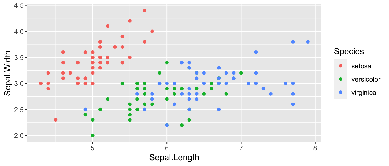

Looking at this graph, it seems that I will likely have a model with different y-intercepts for each species, but it isn’t clear to me if we need different slopes.

We consider the sequence of building successively more complex models:

# make virginica the reference group 
iris <- iris %>%
  mutate( Species = forcats::fct_relevel(Species, 'virginica') )

m1 <- lm( Sepal.Width ~ Sepal.Length, data=iris )            # One line
m2 <- lm( Sepal.Width ~ Sepal.Length + Species, data=iris )  # Parallel Lines
m3 <- lm( Sepal.Width ~ Sepal.Length * Species, data=iris )  # Non-parallel Lines

The three models we consider are the following:

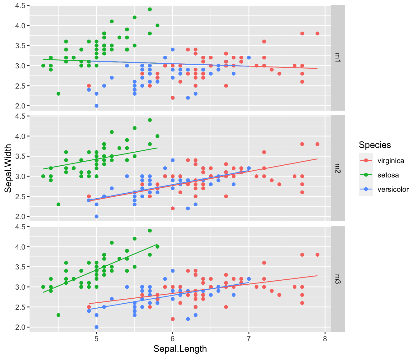
Looking at these, it seems obvious that the simplest model where we ignore Species is horrible. The other two models seem decent, and I am not sure about the parallel lines model vs the differing slopes model.

m1 %>% broom::tidy() %>% mutate_if( is.numeric, round, digits=3 )

## # A tibble: 2 x 5
##   term         estimate std.error statistic p.value
##   <chr>           <dbl>     <dbl>     <dbl>   <dbl>
## 1 (Intercept)     3.42      0.254     13.5    0    
## 2 Sepal.Length   -0.062     0.043     -1.44   0.152

For the simplest model, there is so much unexplained noise that the slope variable isn’t significant.

Moving onto the next most complicated model, where each species has their own y-intercept, but they share a slope, we have

m2 %>% broom::tidy() %>% mutate_if( is.numeric, round, digits=3 )

## # A tibble: 4 x 5
##   term              estimate std.error statistic p.value
##   <chr>                <dbl>     <dbl>     <dbl>   <dbl>
## 1 (Intercept)          0.669     0.308      2.17   0.031
## 2 Sepal.Length         0.35      0.046      7.56   0    
## 3 Speciessetosa        1.01      0.093     10.8    0    
## 4 Speciesversicolor    0.024     0.065      0.37   0.712

The first two lines are the y-intercept and slope associated with the reference group and the last two lines are the y-intercept offsets from the reference group to Setosa and Versicolor, respectively. We have that the slope associated with increasing Sepal Length is significant and that Setosa has a statistically different y-intercept than the reference group Virginica and that Versicolor does not have a statistically different y-intercept than the reference group.

Finally we consider the most complicated model that includes two more slope parameters

m3 %>% broom::tidy() %>% mutate_if( is.numeric, round, digits=3 )

## # A tibble: 6 x 5
##   term                           estimate std.error statistic p.value
##   <chr>                             <dbl>     <dbl>     <dbl>   <dbl>
## 1 (Intercept)                       1.45      0.405     3.57    0    
## 2 Sepal.Length                      0.232     0.061     3.79    0    
## 3 Speciessetosa                    -2.02      0.686    -2.94    0.004
## 4 Speciesversicolor                -0.574     0.605    -0.95    0.344
## 5 Sepal.Length:Speciessetosa        0.567     0.126     4.49    0    
## 6 Sepal.Length:Speciesversicolor    0.088     0.097     0.905   0.367

These parameters are:

Meaning	R-label
Reference group y-intercept	(Intercept)
Reference group slope	Sepal.Length
offset to y-intercept for Setosa	Speciessetosa
offset to y-intercept for Versicolor	Speciesversicolor
offset to slope for Setosa	Sepal.Length:Speciessetosa
offset to slope for Versicolor	Sepal.Length:Speciesversicolor

It appears that slope for Setosa is different from the reference group Virginica. However because we’ve added \(2\) parameters to the model, testing Model2 vs Model3 is not equivalent to just looking at the p-value for that one slope. Instead we need to look at the F-test comparing the two models which will evaluate if the decrease in SSE is sufficient to justify the addition of two parameters.

anova(m2, m3)

## Analysis of Variance Table
## 
## Model 1: Sepal.Width ~ Sepal.Length + Species
## Model 2: Sepal.Width ~ Sepal.Length * Species
##   Res.Df    RSS Df Sum of Sq      F   Pr(>F)    
## 1    146 12.193                                 
## 2    144 10.680  2    1.5132 10.201 7.19e-05 ***
## ---
## Signif. codes:  0 '***' 0.001 '**' 0.01 '*' 0.05 '.' 0.1 ' ' 1

The F-test concludes that there is sufficient decrease in the SSE to justify adding two additional parameters to the model.

5.5 Exercises

The in the faraway package, there is a dataset named phbirths that gives babies birth weights along with their gestational time in utero along with the mother’s smoking status.
1. Load and inspect the dataset using
```
data('phbirths', package='faraway')   # load the data within the package
?faraway::phbirths                    # Look at the help file
```
2. Create a plot of the birth weight vs the gestational age. Color code the points based on the mother’s smoking status. Does it appear that smoking matters?
3. Fit the simple model (one regression line) along with both the main effects (parallel lines) and interaction (non-parallel lines) ANCOVA model to these data. Which model is preferred?
4. Using whichever model you selected in the previous section, create a graph of the data along with the confidence region for the regression line(s).
5. Now consider only the “full term babies” which are babies with gestational age at birth \(\ge 36\) weeks. With this reduced dataset, repeat parts c,d.
6. Interpret the relationship between gestational length and mother’s smoking status on birth weight.
The in the faraway package, there is a dataset named clot that gives information about the time for blood to clot verses the blood dilution concentration when the blood was diluted with prothrombin-free plasma. Unfortunately the researchers had to order the plasma in two different lots (could think of this as two different sources) and need to ascertain if the lot number makes any difference in clotting time.
1. Log transform the time and conc variable and plot the log-transformed data with color of the data point indicating the lot number. (We will discuss why we performed this transformation later in the course.)
2. Ignoring the slight remaining curvature in the data, perform the appropriate analysis using transformed variables. Does lot matter?
In base R, there is a data set ToothGrowth which is data from an experiment giving Vitamin C to guinea pigs. The guinea pigs were given vitamin C doses either via orange juice or an ascorbic acid tablet. The response of interest was a measure of tooth growth where a higher growth is better.
1. Log transform the dose and use that throughout this problem. Use \(e\) as the base, which R does by default when you use the log() function. (We will discuss why we performed this transformation later in the course.)
2. Graph the data, fit appropriate ANCOVA models, and describe the relationship between the delivery method, log(dose) level, and tooth growth. Produce a graph with the data and the regression line(s) along with the confidence region for the line(s).
3. Is there a statistically significant difference in slopes between the two delivery methods?
4. Just using your graphs and visual inspection, at low dose levels, say \(\log(dose)=-0.7\), is there a difference in delivery method? What about at high dose levels, say \(\log(dose)=0.7\)?
5. Use emmeans() to test if there is a statistically significant difference at low dose levels \(\log(dose)=-0.7\). Furthermore, test if there is a statistically significant difference at high dose levels. Summarize your findings.