D. Computer Lab: Analyzing Your Acoustic Data

Part 1. Now it is time to analyze the data you collected for this week’s field lab.

Upload your sound files into either the ‘MyFocalRecordings’ folder or the ’MySoundscapeRecordings’folder and run the code below.

NOTE: Make sure to create the folders if they are not already there and add your sound files!

dir.create(file.path('MyFocalRecordings'), showWarnings = FALSE)
dir.create(file.path('MySoundscapeRecordings'), showWarnings = FALSE)

Part 4a. Your focal recordings

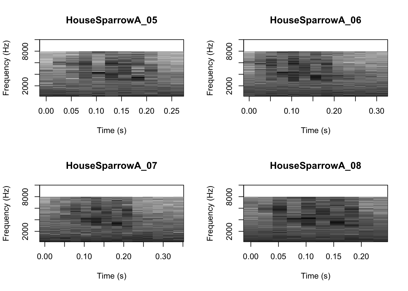
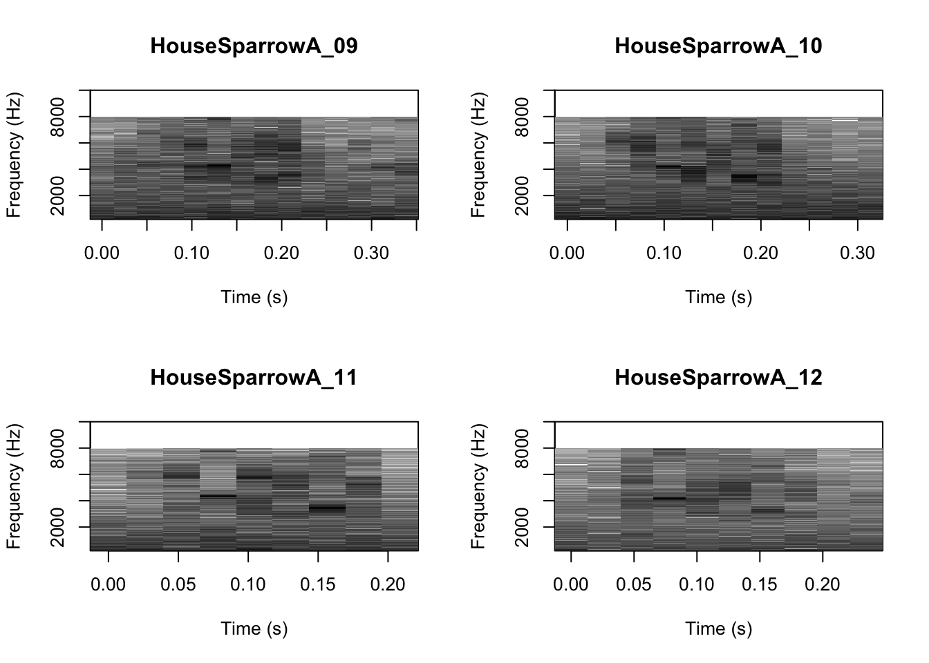
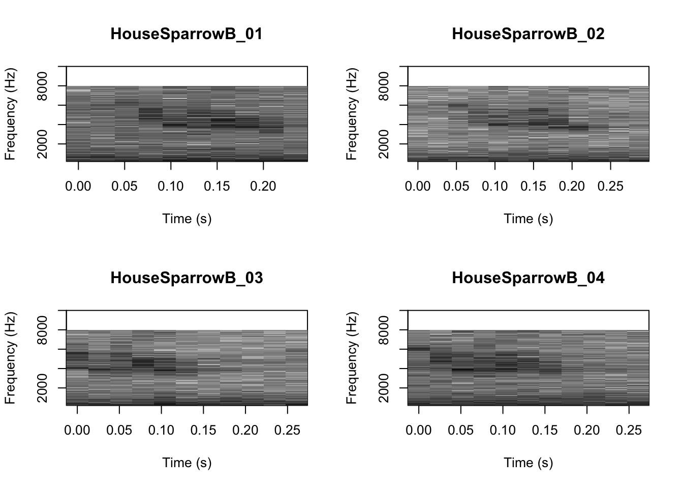
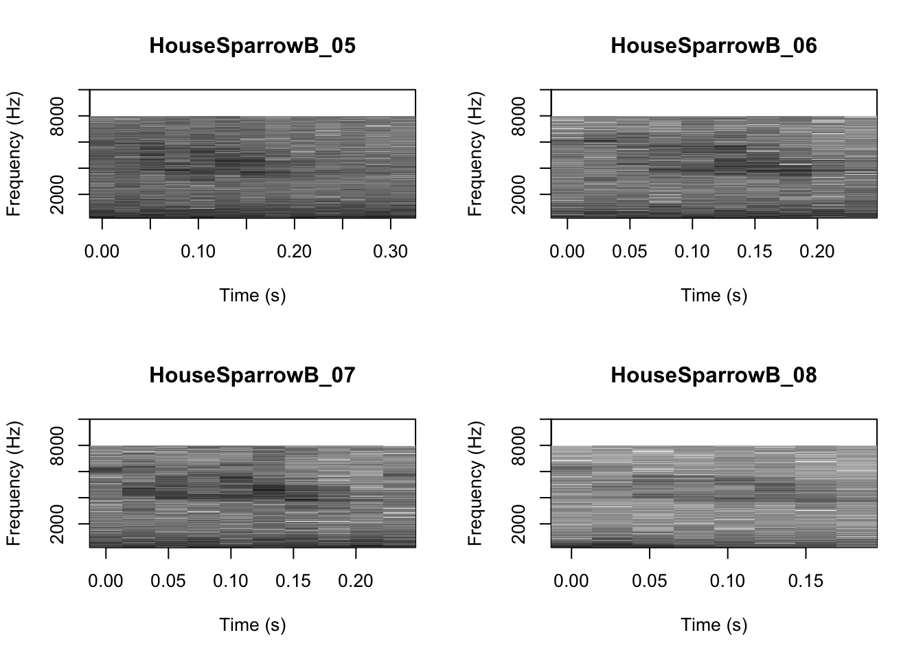
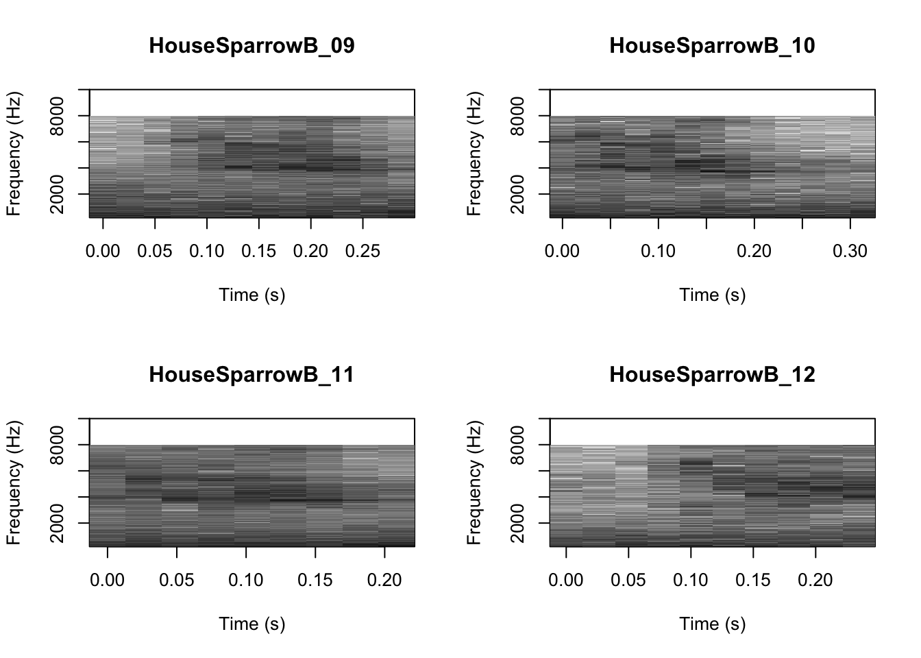
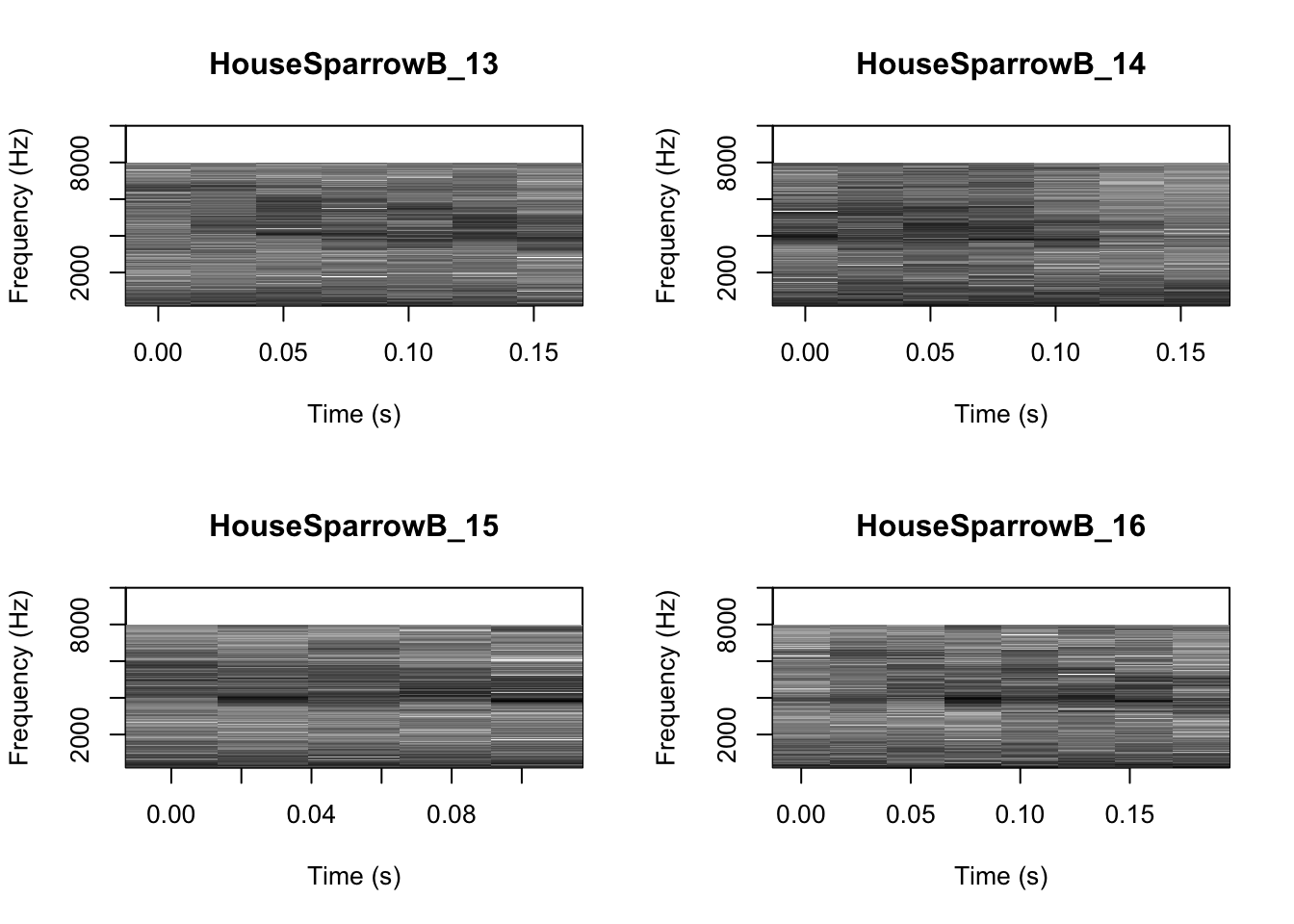
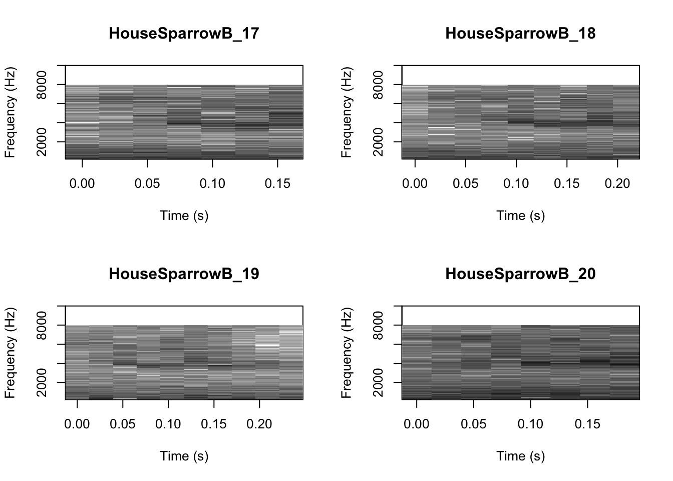
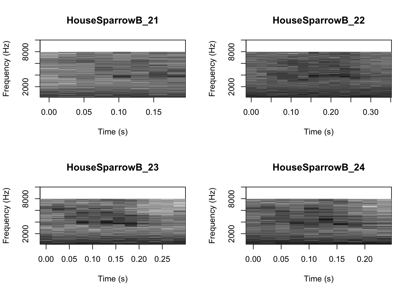
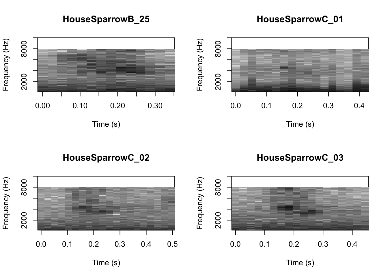
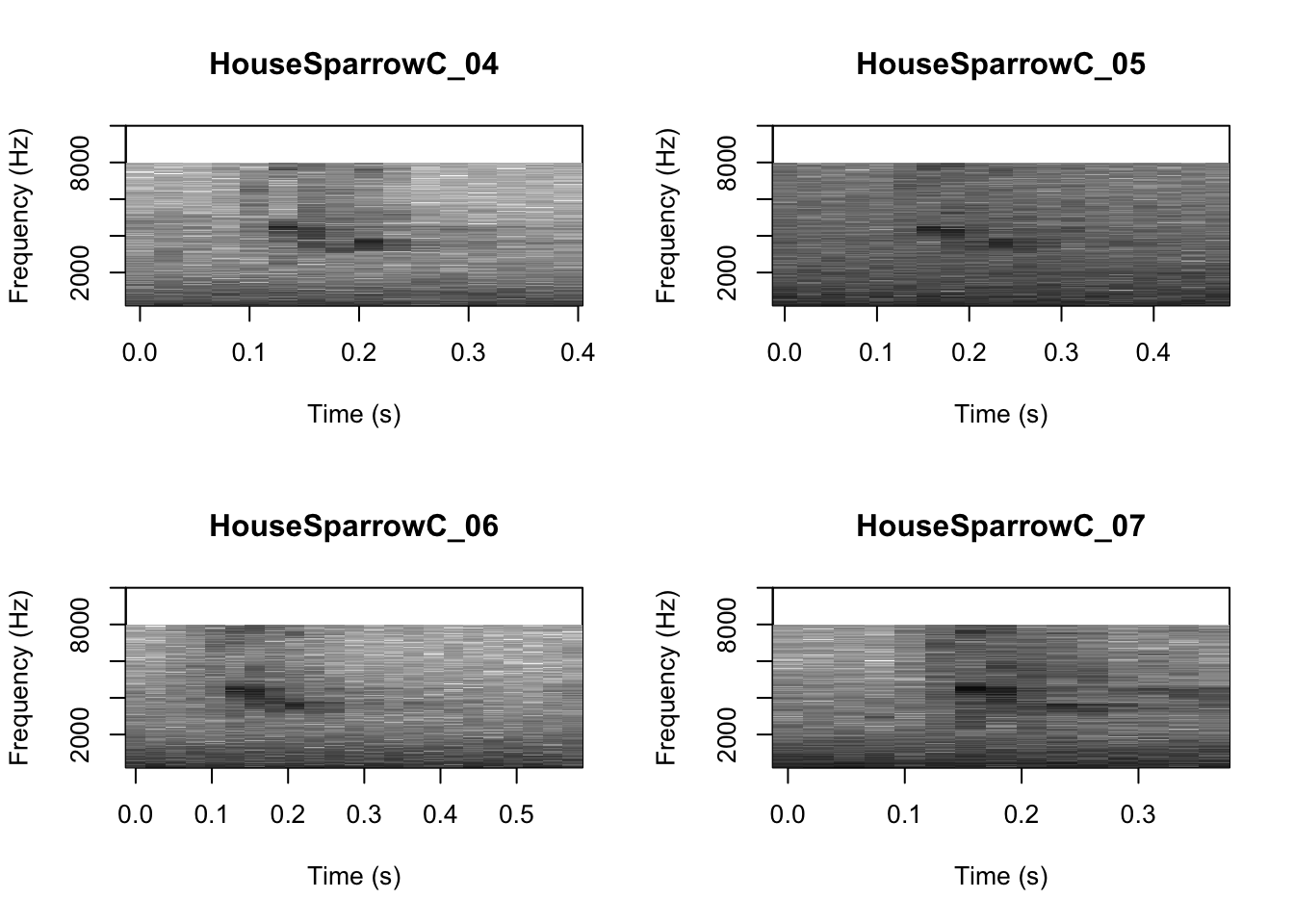
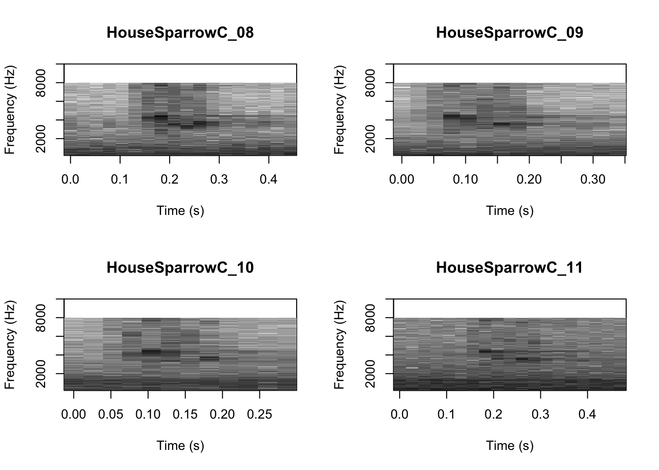
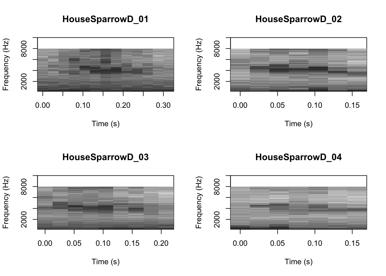
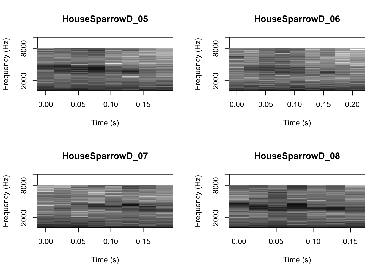
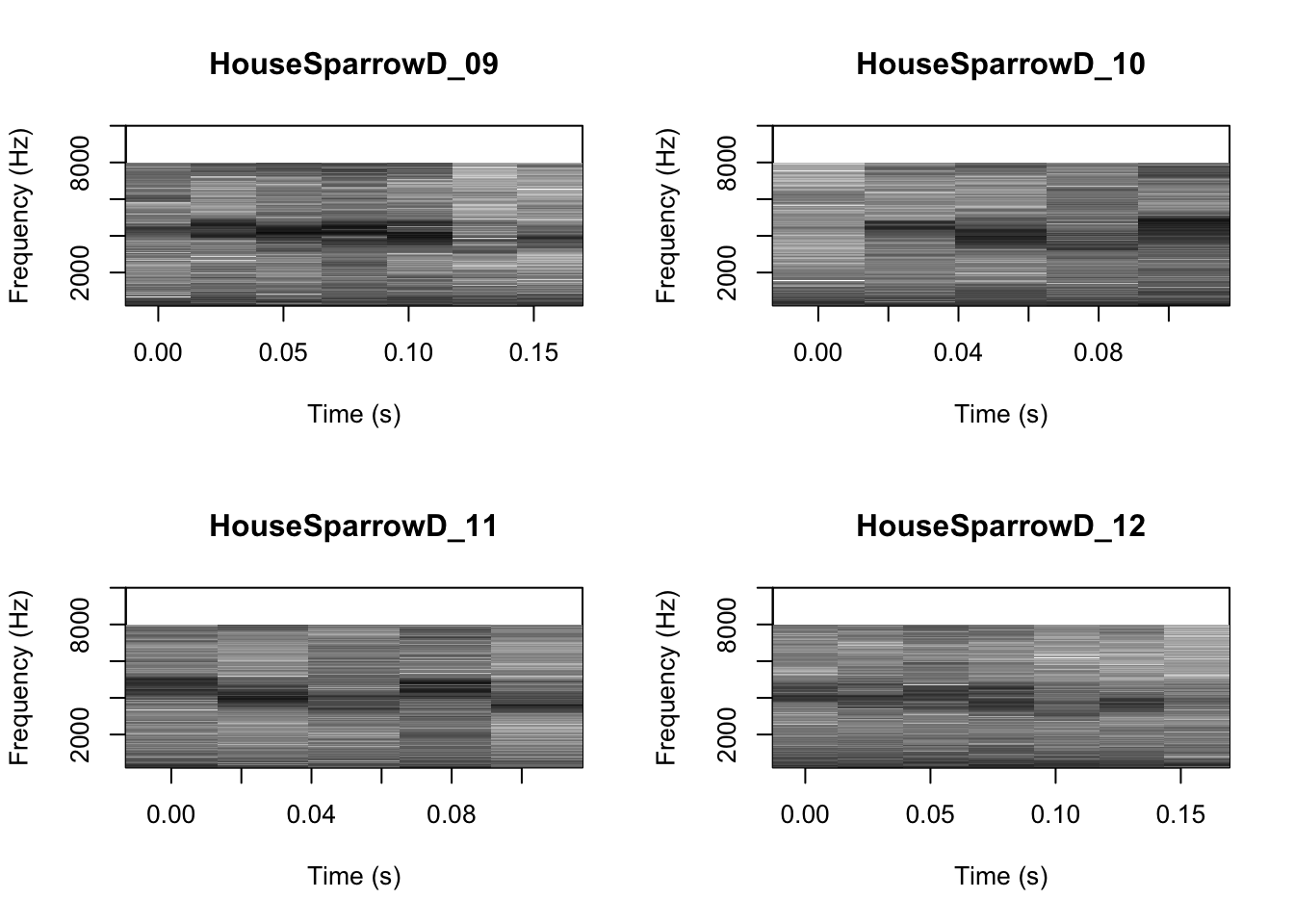
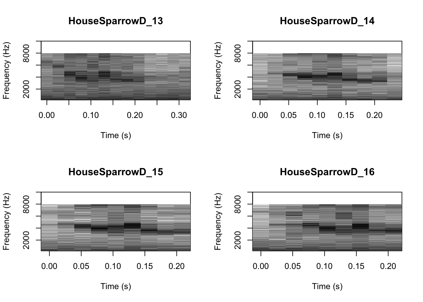
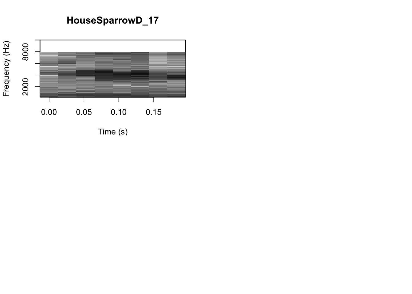
First lets visualize the spectrograms. You may want to change the frequency settings depending on the frequency range of your focal animals.

# We can tell R to print the spectrograms 2x2 using the code below
par(mfrow=c(2,2))

# This is the function to create the spectrograms
SpectrogramFunction(input.dir = "MyFocalRecordings",min.freq = 200,max.freq=10000)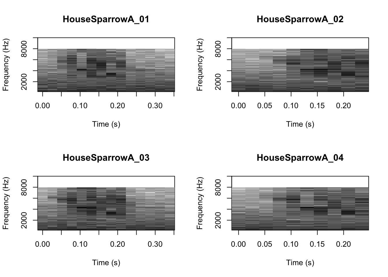

Here is the function to extract the features. Again, based on the frequency range of your focal recordings you may want to change the frequency settings.

MyFeatureDataFrame <- MFCCFunction(input.dir = "MyFocalRecordings",min.freq = 3000,max.freq=7000)

Then we run the principal component analysis

pca_res <- prcomp(MyFeatureDataFrame[,-c(1)], scale. = TRUE)

Now we visualize our results

ggplot2::autoplot(pca_res, data = MyFeatureDataFrame,
         colour = 'Class')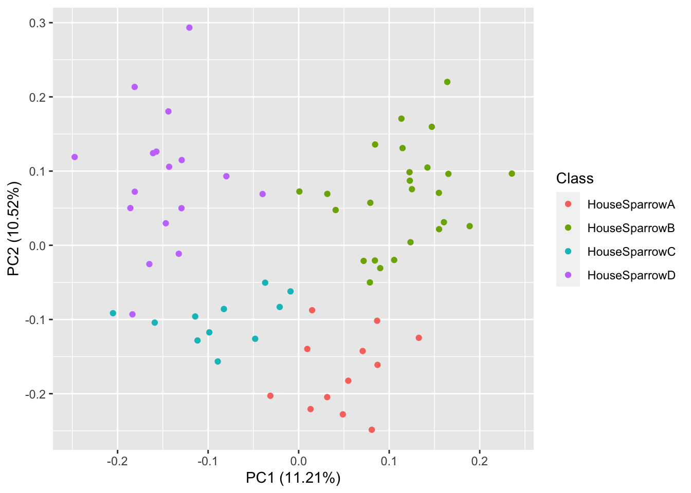

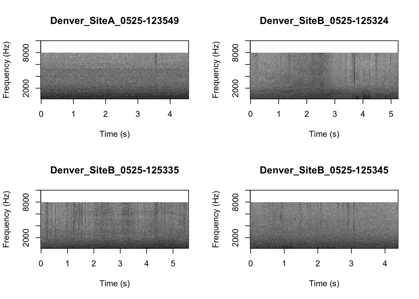
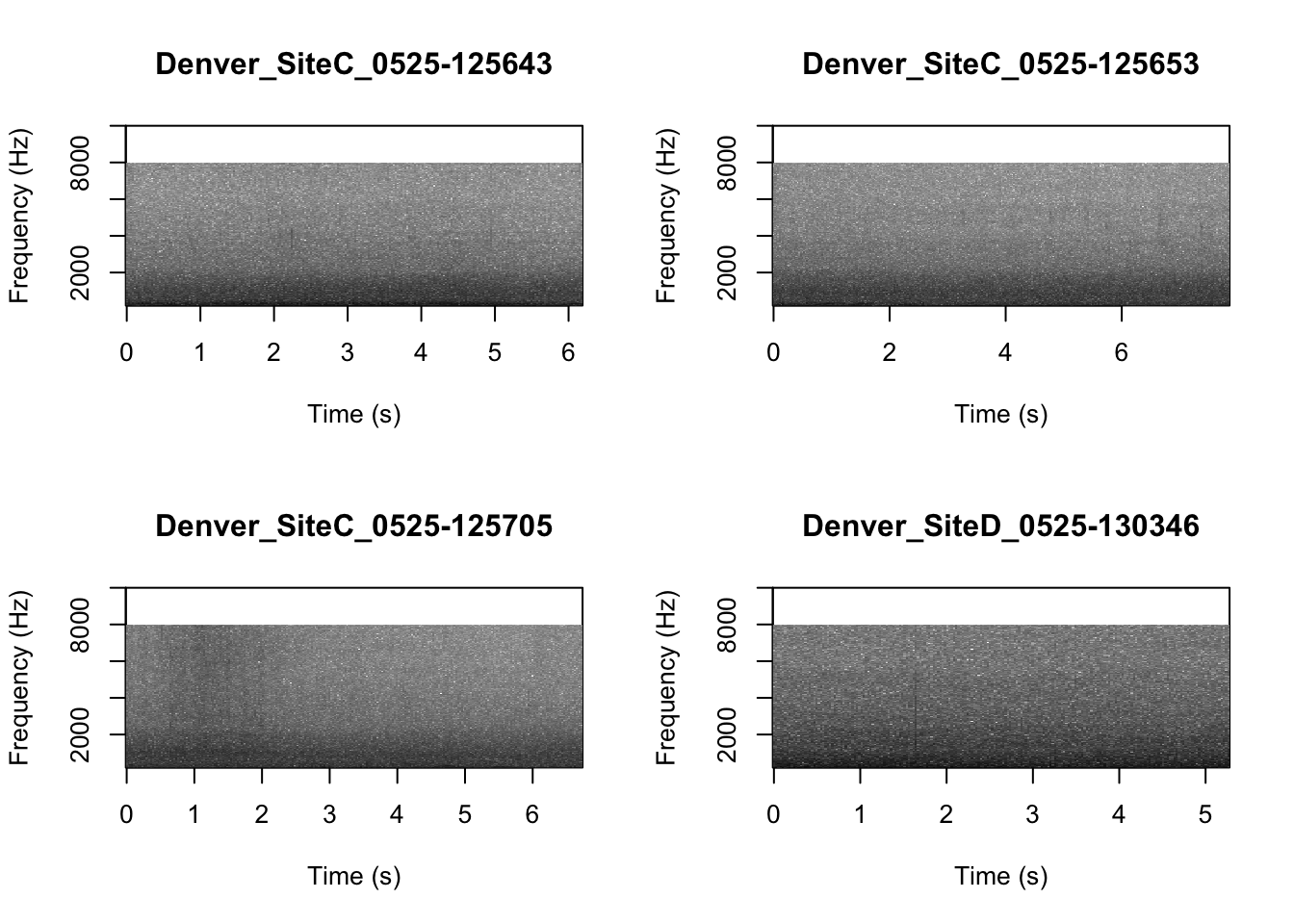
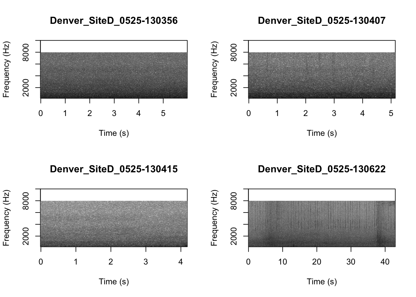
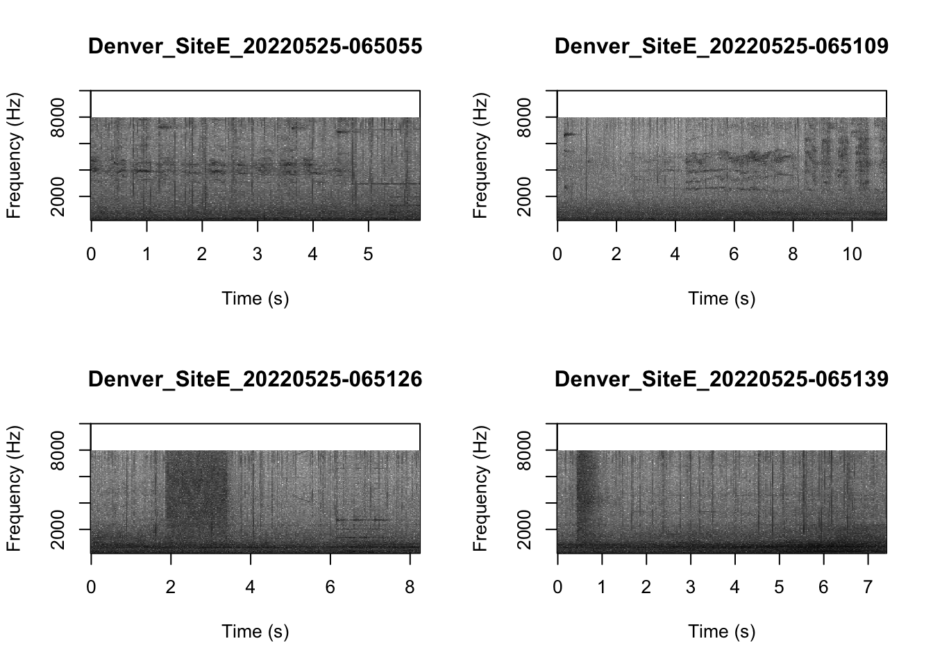
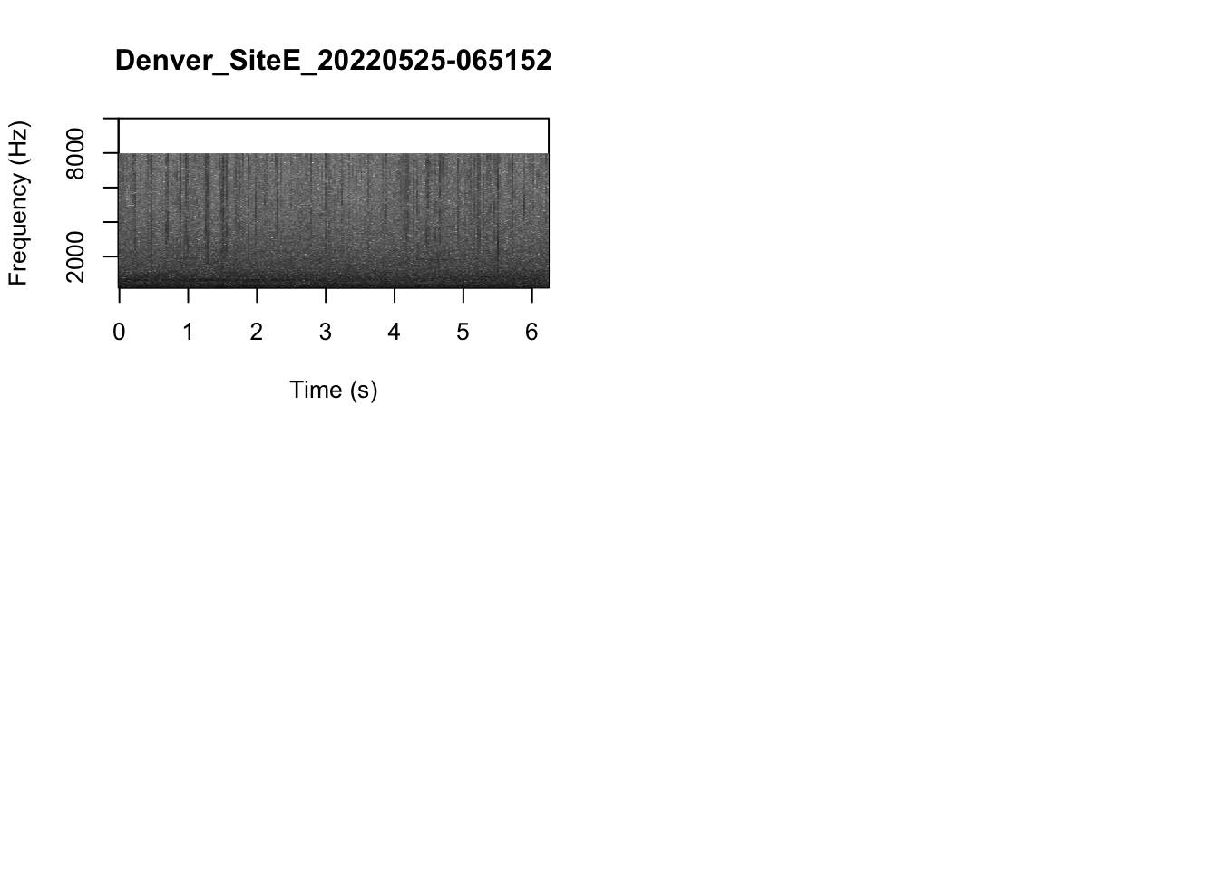
Part 4b. Soundscape recordings

First lets visualize the spectrograms. You probably don’t want to change the frequency settings for this.

# We can tell R to print the spectrograms 2x2 using the code below
par(mfrow=c(2,2))

# This is the function to create the spectrograms
SpectrogramFunction(input.dir = "MySoundscapeRecordings",min.freq = 200,max.freq=10000)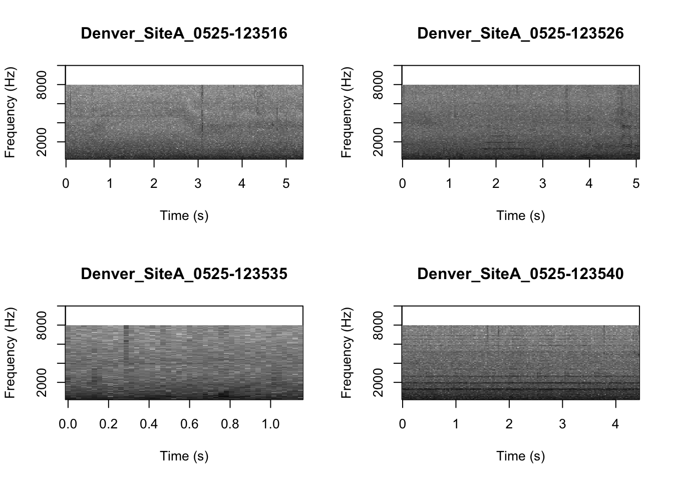

Then we extract the features, which in this case are the MFCCs.

MySoundscapeFeatureDataframe <- 
  MFCCFunctionSite(input.dir = "MySoundscapeRecordings",min.freq = 200,max.freq=10000)

Check the resulting structure of the dataframe to make sure it looks OK.

dim(MySoundscapeFeatureDataframe)

Now we visualize our results

pca_res <- prcomp(MySoundscapeFeatureDataframe[,-c(1)], scale. = TRUE)
ggplot2::autoplot(pca_res, data = MySoundscapeFeatureDataframe, 
         colour = 'Class')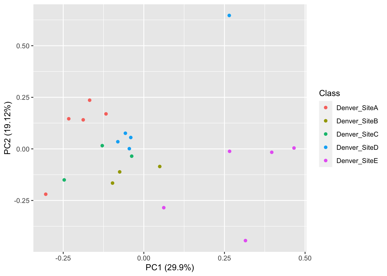

Question 4. Do you see evidence of clustering in either your focal recordings or soundscape recordings?

Question 5.

1.

Sethi, S. S. et al. Characterizing soundscapes across diverse ecosystems using a universal acoustic feature set. Proceedings of the National Academy of Sciences 117, 17049–17055 (2020).

2.

Fischer, J., Noser, R. & Hammerschmidt, K. Bioacoustic field research: A primer to acoustic analyses and playback experiments with primates. American Journal of Primatology 75, 643–663 (2013).

3.

Marten, K. & Marler, P. Sound transmission and its significance for animal vocalization. Behavioral ecology and sociobiology 2, 271–290 (1977).