Computer Lab 6. Analyzing camera trap data.

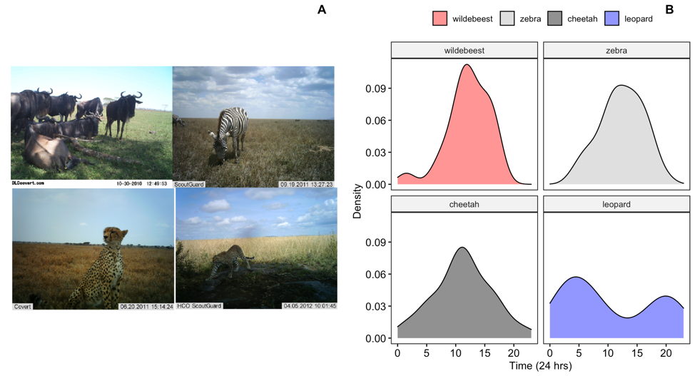
Images of wildebeest, zebra, cheetah and leopard from the Snapshot Serengeti image database (http://lila.science/datasets/snapshot-serengeti)

Figure 6: Images of wildebeest, zebra, cheetah and leopard from the Snapshot Serengeti image database (http://lila.science/datasets/snapshot-serengeti)

Background
In this lab we will use actual camera trap data collected in Serengeti National Park to investigate temporal niche partitioning. The camera trap data that we will use for this field lab comes from the ‘Snapshot Serengeti’ project (http://lila.science/datasets/snapshot-serengeti). The scientists set out out 225 cameras within a 1,125 km2 area. The cameras have been deployed continuously since 2010, and the researchers recruited citizen scientists to help with classifying images (https://www.zooniverse.org/projects/zooniverse/snapshot-serengeti).

Goals of the exercises
The main goal(s) of today’s lab are to:
1) Understand the types of behavioral data that scientists can collect from camera trap photos.
2) Become familiar with one of the ways scientists can compare differences in activity patterns.
3) Think about interspecific interactions of predator-prey and potential competitors in the Serengeti.

Getting started
First we need to load the relevant packages for our data analysis. Packages contain all the functions that are needed for data analysis.

library(behaviouR)
library(ggpubr)

Part 1: Collect Serengeti camera trap data

The original dataset includes over 2.65M sequences of camera trap images (totaling 7.1M images) from ten field seasons. As you can imagine that is a lot of data! For this lab we will focus on a subset of the data collected over the course of a few seasons.

We will be taking random subsets of the camera trap photos (the current default is 5 per season which you should change for your actual study), and we use ‘set.seed’ to make sure that our results are reproducible.

set.seed(2210)

We can use the following code to query the database by season to see which photos are available. The available seasons are 1-4, 6-8,10,11. This function will return a table with all of the available camera trap photos for a particular season. With camera trap data often times photos will be taken in a sequence (e.g. if the animal is moving in front of the camera for a long time). The values in the table below include all photos in a sequence, but the code we use to download the photos only takes the first photo in a sequence. Therefore the sample sizes indicated in this table and the actual sample size may be different.

CameraTrapAnnotations(season = 1)

## 
##        aardvark        aardwolf          baboon     batearedfox 
##             143              88             348             315 
##         buffalo        bushbuck         caracal         cheetah 
##            1455              36              57             575 
##           civet          dikdik           eland        elephant 
##              27             728             113            1687 
##   gazellegrants gazellethomsons           genet         giraffe 
##            4967           29705              28            1923 
##      guineafowl            hare      hartebeest    hippopotamus 
##            3217             327            2139             340 
##     honeybadger    hyenaspotted    hyenastriped          impala 
##              42            2752             112             691 
##          jackal     koribustard         leopard      lionfemale 
##             304             591              38            1519 
##        lionmale        mongoose    monkeyvervet         ostrich 
##             665             290              64             211 
##       otherbird       porcupine        reedbuck        reptiles 
##            2322             114             946             357 
##      rhinoceros         rodents   secretarybird          serval 
##               6             129             198             174 
##            topi         warthog       waterbuck         wildcat 
##             428            2685              25              48 
##      wildebeest           zebra         zorilla 
##             689            5592               9

For this lab you are going to choose two animals from the camera trap dataset. It could be a pair of animals that are predator and prey or two potential competitors. Once you decide on the two animals you want to compare you will make some predictions about how you think they will differ in their activity patterns.

Now we will use another function to download the camera trap photos and save them locally to our computer. You can change the season by changing the values for season (remember the available seasons are 1-4, 6-8,10,11). You can change the focal animal by changing the ‘AnimalID’; make sure that the spelling and case is exactly the same as in the table above. You can change the number of photos per season that you download (the default is 5). When ‘create.dir’ is true this will create a folder in your current working directory. For this example the folder is called ‘CameraTrapPhotoszebra’. If create.dir=‘FALSE’ all the photos will be downloaded directly to your working directory. To find the directory type ‘getwd()’ into your R console.

CombinedAnimalDF <- CameraTrapDataAccess(urlpath= 'https://lilablobssc.blob.core.windows.net/snapshotserengeti-unzipped/',
                     season= list(1,2),AnimalID='zebra', NumPhotos= 5,create.dir=TRUE)

Here we isolate only the columns from the dataframe that we need.

CombinedAnimalDF <- CombinedAnimalDF[,c("category_id","season","location","filename")]
head(CombinedAnimalDF)

##       category_id season location
## 1975        zebra     S1      C03
## 4742        zebra     S1      C06
## 292         zebra     S1      B05
## 7513        zebra     S1      D05
## 4582        zebra     S1      C06
## 45467       zebra     S2      E02
##                                     filename
## 1975  CameraTrapPhotoszebra/zebra_S1_C03.JPG
## 4742  CameraTrapPhotoszebra/zebra_S1_C06.JPG
## 292   CameraTrapPhotoszebra/zebra_S1_B05.JPG
## 7513  CameraTrapPhotoszebra/zebra_S1_D05.JPG
## 4582  CameraTrapPhotoszebra/zebra_S1_C06.JPG
## 45467 CameraTrapPhotoszebra/zebra_S2_E02.JPG

The function below will allow you to enter data and look through each photo included in the ‘CombinedAnimalDF’ spreadsheet and enter the time that the photo was taken. You can change option=‘Plot’ to option=‘Viewer’ to load the photos more quickly, but you will have to expand the photo to see the whole thing. The input file should be the dataframe created using the ‘CameraTrapDataAccess’ function. You can break out of the function at any time by typing ‘break’. It will print out which row of the dataframe you were on when you stopped the function. If you would like to resume where you left off you must change ‘rowstart=1’ to the row number indicated, and change ‘dataframe.cont = FALSE’ to ‘dataframe.cont = TRUE’.

Here is the function to view photos and annotate data.

CombinedAnimalDF_TimeAdded <- CameraTrapDataCollection(inputfile = CombinedAnimalDF, 
                                                       rowstart = 1, dataframe.cont = FALSE, option = "Viewer")

Now you may want to save your datasheet locally

write.csv(CombinedAnimalDF_TimeAdded,'CombinedAnimalDF_TimeAdded.csv',row.names = F)

Part 2: Analyze your Serengeti camera trap data

First we load your data sheet with the times added. NOTE: Make sure that your updated datasheet has the exact same name as the file indicated below.

# You can read in your datasheet that you saved
CombinedDFTimes <- read.csv('CombinedAnimalDF_TimeAdded.csv')

Then we can check the structure

head(CombinedDFTimes)

Now we can make a density plot that will show the distribution of camera trap photos that were taken over 24-hours. We add the fill = ‘category_id’ so that we show different distributions for each animal.

ggpubr::ggdensity(data=CombinedDFTimes,x='Time',fill = 'category_id')+
  xlab('Time (24 hrs)') +ylab('Density')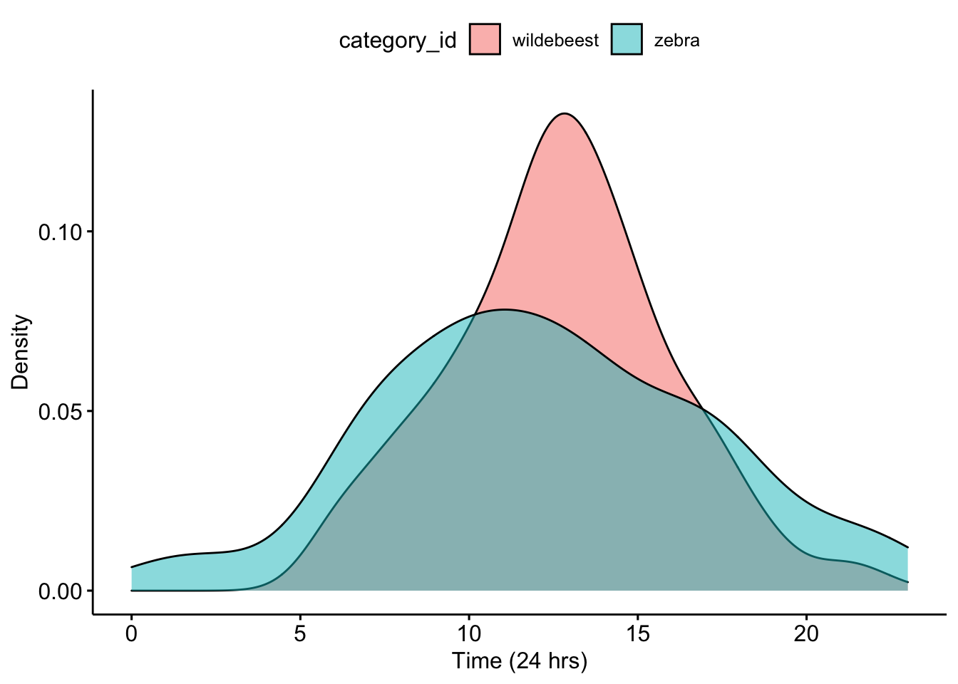

Question 1. What do you notice about the overlap of the two density curves? Does it look like there is temporal niche partitioning?

Now we can calculate an overlap coefficient which can be used to investigate potential competitive and interaction possibilities between species.The value ranges from ranges from 0 (no overlap) to 1 (complete overlap).

First we subset our data to focus on the first animal in our dataset

FirstAnimal <- subset(CombinedDFTimes,category_id=='zebra')

Then we subset our data to focus on the second animal in our dataset

SecondAnimal <- subset(CombinedDFTimes,category_id=='wildebeest')

Now we use the overlap function to calculate the overlap coefficient

bayestestR::overlap(FirstAnimal$Time,SecondAnimal$Time)

## # Overlap
## 
## 0.81

Question 2. How do you interpret the overlap coefficient for your data?

Part 3: Focus on your partner’s Serengeti camera trap data

Now we will read in our partners data.
NOTE: Make sure that your updated datasheet has the exact same name as the file indicated below.

CombinedPartnerDFTimes <- read.csv('CombinedAnimalDF_TimeAddedPartner.csv')

Let’s check the structure

head(CombinedPartnerDFTimes)

##   category_id season location
## 1     leopard     S1      B06
## 2     leopard     S1      D06
## 3     leopard     S1      D06
## 4     leopard     S1      D06
## 5     leopard     S1      E06
## 6     leopard     S1      E06
##                                     filename Time
## 1 CameraTrapPhotosleopard/leopard_S1_B06.JPG    4
## 2 CameraTrapPhotosleopard/leopard_S1_D06.JPG   20
## 3 CameraTrapPhotosleopard/leopard_S1_D06.JPG   20
## 4 CameraTrapPhotosleopard/leopard_S1_D06.JPG   20
## 5 CameraTrapPhotosleopard/leopard_S1_E06.JPG    4
## 6 CameraTrapPhotosleopard/leopard_S1_E06.JPG    4

Now we can make a density plot for our partner’s data.

ggpubr::ggdensity(data=CombinedPartnerDFTimes,x='Time',fill = 'category_id')+
  xlab('Time (24 hrs)') +ylab('Density')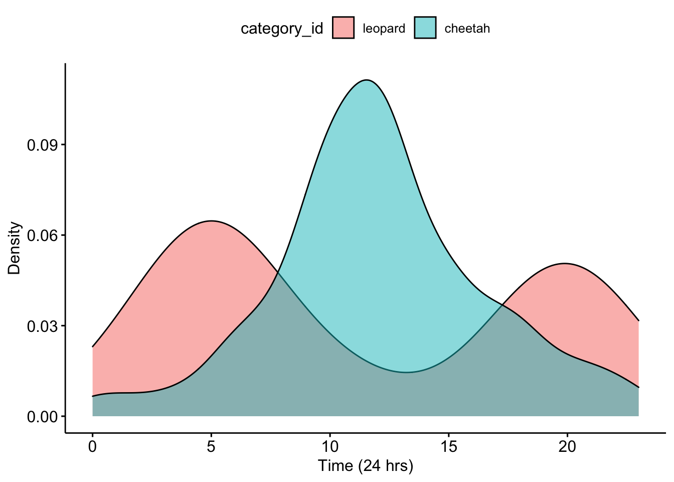

Question 3. What do you notice about the overlap of the two density curves for your partner’s data? Does it look like there is temporal niche partitioning?

First we subset our data to focus on the first animal in your partner’s data set

FirstAnimalPartner <- subset(CombinedPartnerDFTimes,category_id=='cheetah')

Then we subset our data to focus on the second animal in our dataset

SecondAnimalPartner <- subset(CombinedPartnerDFTimes,category_id=='leopard')

Now we use the overlap function to calculate the overlap coefficient

bayestestR::overlap(FirstAnimalPartner$Time,SecondAnimalPartner$Time)

## # Overlap
## 
## 0.44

Question 4. What is the overlap coefficient for your partner’s data? How do you interpret this?

Part 4. Investigating temporal niche partitioning in four different animals

First we combine both datasets

AllDataCombined <- rbind.data.frame(CombinedDFTimes,CombinedPartnerDFTimes)

Then we plot the diel activity patterns for all four species

ggpubr::ggdensity(data=AllDataCombined,x='Time',fill = 'category_id',facet.by = 'category_id')+
  xlab('Time (24 hrs)') +ylab('Density')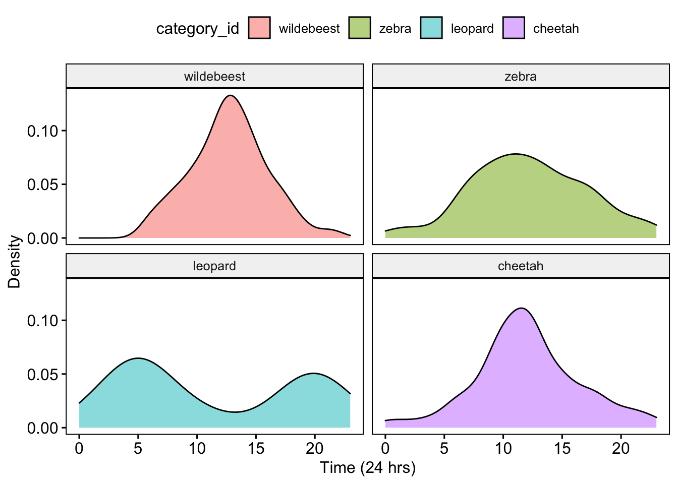

Question 5. Based on the activity patterns and your understanding of the Serengeti food web how do you interpret these results? Is there evidence of temporal niche partitioning among potential competitors? What about interactions between potential predators and prey?