Chapter 5 Data Analysis

5.1 Descriptive statistics

5.1.1 Univariate analysis

Index of qualitative variation (categorical variables)

R

freq(allbus2012$female)

## Frequencies  
## allbus2012$female  
## Type: Factor  
## 
##                Freq   % Valid   % Valid Cum.   % Total   % Total Cum.
## ------------ ------ --------- -------------- --------- --------------
##         Male   1725     49.57          49.57     49.57          49.57
##       Female   1755     50.43         100.00     50.43         100.00
##         <NA>      0                               0.00         100.00
##        Total   3480    100.00         100.00    100.00         100.00

freq(allbus2012$migrant)

## Frequencies  
## allbus2012$migrant  
## Type: Factor  
## 
##                 Freq   % Valid   % Valid Cum.   % Total   % Total Cum.
## ------------- ------ --------- -------------- --------- --------------
##        Native   3298     94.77          94.77     94.77          94.77
##       Migrant    182      5.23         100.00      5.23         100.00
##          <NA>      0                               0.00         100.00
##         Total   3480    100.00         100.00    100.00         100.00

Measures of central tendency (metric variables)

The most important measures of central tendency are the arithmetic mean, the median, and the mode.

R

allbus2012 %>% 
    select(class, imp_nei, imp_fr, imp_fam, health, finance, lifesat) %>% 
    descr(stats = c("min", "max", "med", "mean"), transpose = T)

## Descriptive Statistics  
## allbus2012  
## Label: GGSScompact 2012  
## N: 3480  
## 
##                  Min     Max   Median   Mean
## ------------- ------ ------- -------- ------
##         class   1.00    5.00     3.00   2.77
##       finance   1.00    5.00     4.00   3.53
##        health   1.00    5.00     4.00   3.55
##       imp_fam   1.00    7.00     7.00   6.50
##        imp_fr   1.00    7.00     6.00   5.68
##       imp_nei   1.00    7.00     5.00   4.60
##       lifesat   1.00   11.00     9.00   8.64

freq(allbus2012$lifesat)

## Frequencies  
## allbus2012$lifesat  
## Type: Numeric  
## 
##               Freq   % Valid   % Valid Cum.   % Total   % Total Cum.
## ----------- ------ --------- -------------- --------- --------------
##           1      8      0.23           0.23      0.23           0.23
##           2      6      0.17           0.40      0.17           0.40
##           3     26      0.75           1.15      0.75           1.15
##           4     46      1.32           2.47      1.32           2.47
##           5     76      2.19           4.66      2.18           4.66
##           6    283      8.14          12.80      8.13          12.79
##           7    263      7.56          20.36      7.56          20.34
##           8    606     17.43          37.79     17.41          37.76
##           9   1071     30.80          68.59     30.78          68.53
##          10    653     18.78          87.37     18.76          87.30
##          11    439     12.63         100.00     12.61          99.91
##        <NA>      3                               0.09         100.00
##       Total   3480    100.00         100.00    100.00         100.00

Measures of dispersion (metric variables)

R

Variance, standard deviation (sd), coefficient of variation (sd/mean)

allbus2012 %>% 
    select(class, starts_with("imp"), health, finance, lifesat) %>% 
    descr(stats = c("min", "max", "med", "mean", "sd", "cv"), transpose = T)

## Descriptive Statistics  
## allbus2012  
## Label: GGSScompact 2012  
## N: 3480  
## 
##                  Min     Max   Median   Mean   Std.Dev     CV
## ------------- ------ ------- -------- ------ --------- ------
##         class   1.00    5.00     3.00   2.77      0.66   0.24
##       finance   1.00    5.00     4.00   3.53      0.80   0.23
##        health   1.00    5.00     4.00   3.55      1.00   0.28
##       imp_fam   1.00    7.00     7.00   6.50      1.15   0.18
##        imp_fr   1.00    7.00     6.00   5.68      1.19   0.21
##       imp_nei   1.00    7.00     5.00   4.60      1.59   0.35
##       lifesat   1.00   11.00     9.00   8.64      1.72   0.20

5-point statistics (see, Tuckey 1975)

allbus2012 %>% 
    select(class, starts_with("imp"), health, finance, lifesat) %>% 
    descr(stats = c("fivenum"), transpose = T)

## Descriptive Statistics  
## allbus2012  
## Label: GGSScompact 2012  
## N: 3480  
## 
##                  Min     Q1   Median      Q3     Max
## ------------- ------ ------ -------- ------- -------
##         class   1.00   2.00     3.00    3.00    5.00
##       finance   1.00   3.00     4.00    4.00    5.00
##        health   1.00   3.00     4.00    4.00    5.00
##       imp_fam   1.00   7.00     7.00    7.00    7.00
##        imp_fr   1.00   5.00     6.00    7.00    7.00
##       imp_nei   1.00   4.00     5.00    6.00    7.00
##       lifesat   1.00   8.00     9.00   10.00   11.00

Skewness and kurtosis

allbus2012 %>% 
    select(class, starts_with("imp"), health, finance, lifesat) %>% 
    descr(stats = c("min", "max", "med", "mean", "skewness", "kurtosis"), 
          transpose = T)

## Descriptive Statistics  
## allbus2012  
## Label: GGSScompact 2012  
## N: 3480  
## 
##                  Min     Max   Median   Mean   Skewness   Kurtosis
## ------------- ------ ------- -------- ------ ---------- ----------
##         class   1.00    5.00     3.00   2.77      -0.05       0.54
##       finance   1.00    5.00     4.00   3.53      -0.83       0.74
##        health   1.00    5.00     4.00   3.55      -0.47      -0.20
##       imp_fam   1.00    7.00     7.00   6.50      -2.89       8.67
##        imp_fr   1.00    7.00     6.00   5.68      -0.84       0.48
##       imp_nei   1.00    7.00     5.00   4.60      -0.35      -0.52
##       lifesat   1.00   11.00     9.00   8.64      -0.98       1.33

Histogram and box-plot

ggplot(allbus2012, aes(x = lifesat)) +
    geom_histogram() +
    labs(title = "Life satisfaction") +
    scale_x_continuous(breaks = 1:11) +
    theme_stata(scheme = "s1mono")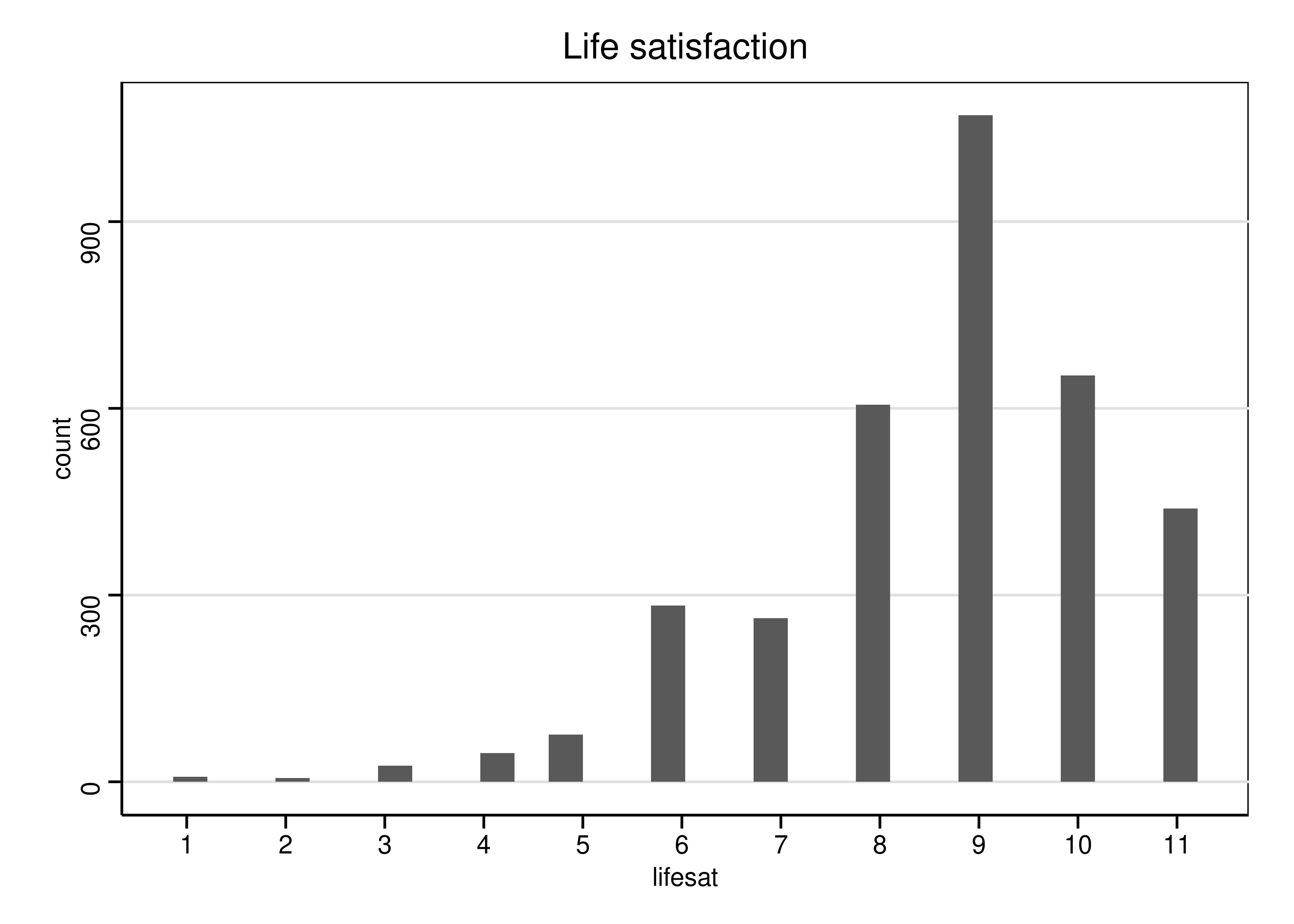

ggplot(allbus2012, aes(x = female, y = lifesat)) +
    geom_boxplot() +
    labs(x = "", y = "Life satisfaction") +
    theme_stata(scheme = "s1mono")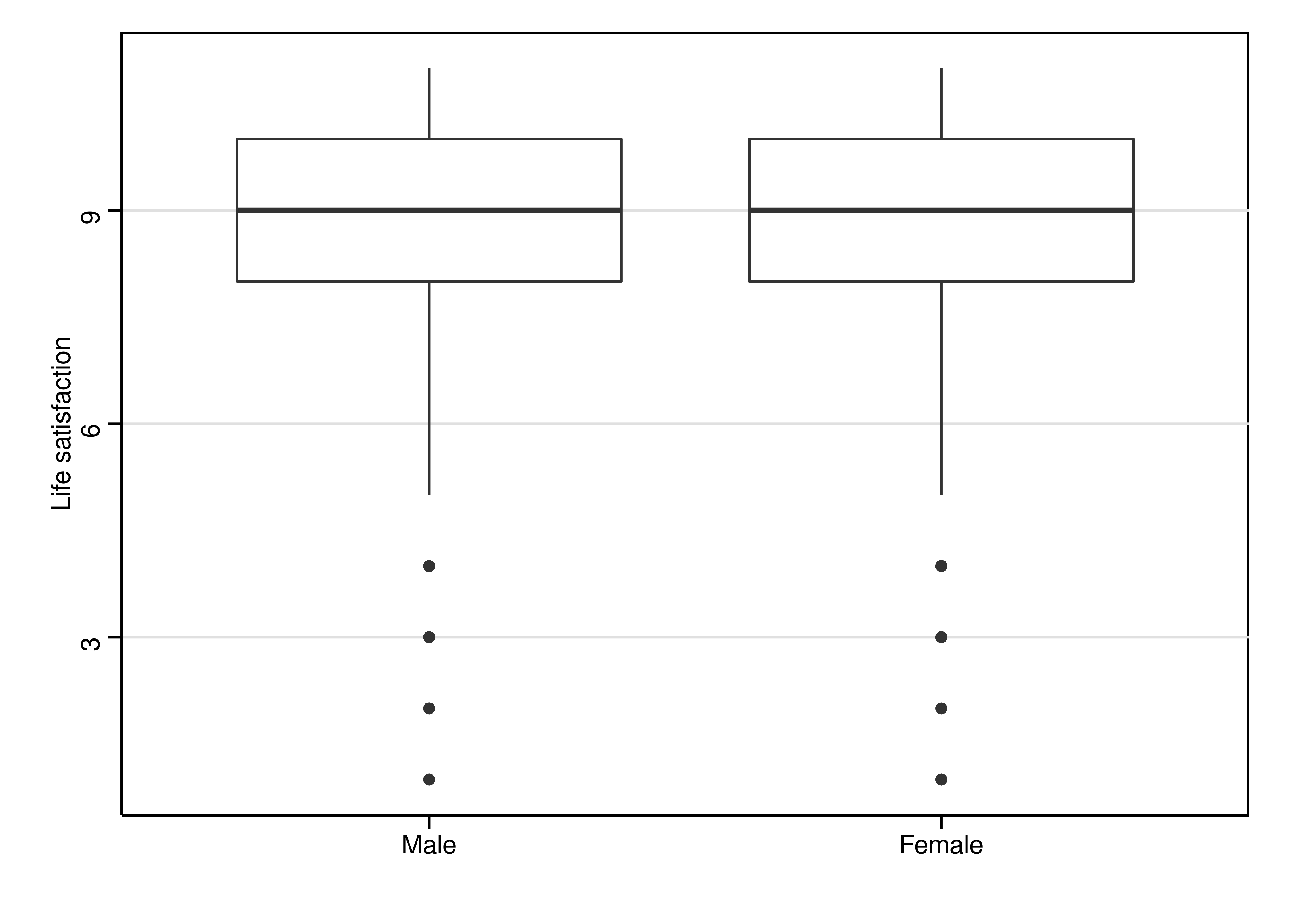

5.1.2 Bivariate analysis

Categorical characteristics: Chi2 und Cramer’s V

R

ctable(allbus2012$female, allbus2012$migrant,
       prop = "none")

## Cross-Tabulation  
## female * migrant  
## Data Frame: allbus2012  
## Label: GGSScompact 2012  
## 
## -------- --------- -------- --------- -------
##            migrant   Native   Migrant   Total
##   female                                     
##     Male               1643        82    1725
##   Female               1655       100    1755
##    Total               3298       182    3480
## -------- --------- -------- --------- -------

allbus2012 %>% 
    crosstable_statistics(female, migrant, 
                          statistics = "cramer",
                          correct = FALSE)

## 
## # Measure of Association for Contingency Tables
## 
##   Chi-squared: 1.5654
##    Cramer's V: 0.0212
##       p-value: 0.2109

ctable(allbus2012$female, allbus2012$astrology,
       prop = "none")

## Cross-Tabulation  
## female * astrology  
## Data Frame: allbus2012  
## Label: GGSScompact 2012  
## 
## -------- ----------- ------ ----- ------ -------
##            astrology     No   Yes   <NA>   Total
##   female                                        
##     Male               1431   290      4    1725
##   Female               1245   506      4    1755
##    Total               2676   796      8    3480
## -------- ----------- ------ ----- ------ -------

allbus2012 %>% 
    crosstable_statistics(female, astrology, 
                          statistics = "cramer",
                          correct = FALSE)

## 
## # Measure of Association for Contingency Tables
## 
##   Chi-squared: 71.2874
##    Cramer's V: 0.1433
##       p-value: <0.001

Metric and categorical

R

t.test(allbus2012$lifesat ~ allbus2012$female,
       var.equal = TRUE)

## 
## 	Two Sample t-test
## 
## data:  allbus2012$lifesat by allbus2012$female
## t = -1.9648, df = 3475, p-value = 0.04951
## alternative hypothesis: true difference in means is not equal to 0
## 95 percent confidence interval:
##  -0.2288332507 -0.0002433446
## sample estimates:
##   mean in group Male mean in group Female 
##             8.583865             8.698404

Metric and metric

R

allbus2012 %>% 
    select(lifesat, finance, health, class) %>% 
    correlation()

## Parameter1 | Parameter2 |    r |       95% CI |     t |   df |      p |  Method | n_Obs
## ---------------------------------------------------------------------------------------
## lifesat    |    finance | 0.44 | [0.42, 0.47] | 29.24 | 3471 | < .001 | Pearson |  3473
## lifesat    |     health | 0.31 | [0.28, 0.34] | 19.49 | 3473 | < .001 | Pearson |  3475
## lifesat    |      class | 0.24 | [0.21, 0.27] | 14.35 | 3428 | < .001 | Pearson |  3430
## finance    |     health | 0.23 | [0.20, 0.26] | 14.07 | 3472 | < .001 | Pearson |  3474
## finance    |      class | 0.34 | [0.31, 0.37] | 21.35 | 3427 | < .001 | Pearson |  3429
## health     |      class | 0.19 | [0.16, 0.23] | 11.52 | 3429 | < .001 | Pearson |  3431

5.2 Inferential statistics

5.2.1 Linear regression

OLS-regression and diagnostics

R

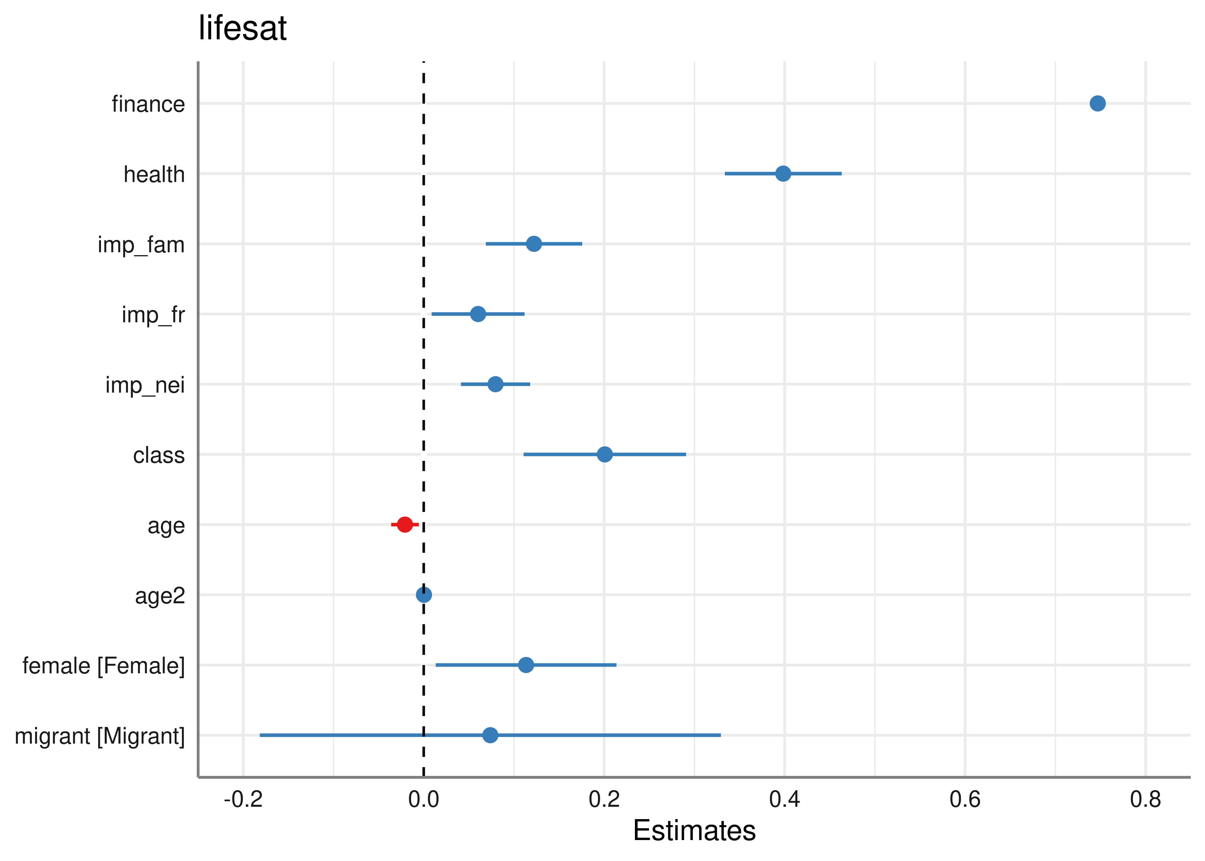
ols <- lm(lifesat ~ finance + health + imp_fam + imp_fr + imp_nei + 
              class + age + age2 + female + migrant,
          data = allbus2012)

tab_model(ols, show.se = TRUE, digits = 3)

	lifesat
Predictors	Estimates	std. Error	CI	p
(Intercept)	2.772	0.298	2.188 – 3.356	<0.001
finance	0.747	0.035	0.679 – 0.815	<0.001
health	0.398	0.028	0.344 – 0.453	<0.001
imp_fam	0.122	0.023	0.078 – 0.167	<0.001
imp_fr	0.060	0.023	0.015 – 0.105	0.009
imp_nei	0.080	0.018	0.045 – 0.114	<0.001
class	0.201	0.041	0.121 – 0.281	<0.001
age	-0.021	0.008	-0.036 – -0.005	0.008
age2	0.000	0.000	0.000 – 0.000	0.001
female [Female]	0.113	0.051	0.013 – 0.214	0.026
migrant [Migrant]	0.074	0.115	-0.153 – 0.300	0.523
Observations	3407
R2 / R2 adjusted	0.270 / 0.268

ols_test_breusch_pagan(ols)

## 
##  Breusch Pagan Test for Heteroskedasticity
##  -----------------------------------------
##  Ho: the variance is constant            
##  Ha: the variance is not constant        
## 
##                Data                 
##  -----------------------------------
##  Response : lifesat 
##  Variables: fitted values of lifesat 
## 
##          Test Summary           
##  -------------------------------
##  DF            =    1 
##  Chi2          =    257.3509 
##  Prob > Chi2   =    6.485887e-58

resettest(ols, power = 2:4, type = "fitted", data = allbus2012)

## 
## 	RESET test
## 
## data:  ols
## RESET = 0.5925, df1 = 3, df2 = 3393, p-value = 0.6199

Heteroskedasticity robust standard errors

Due to heteroskedasticity robust standard errors should be estimated

R

tab_model(ols, vcov.fun = "HC", vcov.type = "HC1",
                  show.se = TRUE, digits = 3)

	lifesat
Predictors	Estimates	std. Error	CI	p
(Intercept)	2.772	0.324	2.137 – 3.407	<0.001
finance	0.747	0.041	0.666 – 0.828	<0.001
health	0.398	0.033	0.334 – 0.463	<0.001
imp_fam	0.122	0.027	0.069 – 0.176	<0.001
imp_fr	0.060	0.026	0.009 – 0.112	0.022
imp_nei	0.080	0.020	0.041 – 0.118	<0.001
class	0.201	0.046	0.111 – 0.291	<0.001
age	-0.021	0.008	-0.036 – -0.005	0.008
age2	0.000	0.000	0.000 – 0.000	0.001
female [Female]	0.113	0.051	0.013 – 0.214	0.026
migrant [Migrant]	0.074	0.130	-0.182 – 0.329	0.571
Observations	3407
R2 / R2 adjusted	0.270 / 0.268

Standardized b-coefficients

One can also request standardized b-coefficients (betas) to compare the strength of relation between coefficients.

R

tab_model(ols, show.se = TRUE, show.std = TRUE,
          digits = 3)

	lifesat
Predictors	Estimates	std. Error	std. Beta	standardized std. Error	CI	standardized CI	p
(Intercept)	2.772	0.298	-0.036	0.021	2.188 – 3.356	-0.077 – 0.006	<0.001
finance	0.747	0.035	0.348	0.016	0.679 – 0.815	0.316 – 0.380	<0.001
health	0.398	0.028	0.233	0.016	0.344 – 0.453	0.201 – 0.265	<0.001
imp_fam	0.122	0.023	0.081	0.015	0.078 – 0.167	0.052 – 0.111	<0.001
imp_fr	0.060	0.023	0.041	0.016	0.015 – 0.105	0.011 – 0.072	0.009
imp_nei	0.080	0.018	0.074	0.016	0.045 – 0.114	0.042 – 0.106	<0.001
class	0.201	0.041	0.078	0.016	0.121 – 0.281	0.047 – 0.109	<0.001
age	-0.021	0.008	-0.215	0.081	-0.036 – -0.005	-0.374 – -0.056	0.008
age2	0.000	0.000	0.275	0.081	0.000 – 0.000	0.117 – 0.433	0.001
female [Female]	0.113	0.051	0.066	0.030	0.013 – 0.214	0.008 – 0.125	0.026
migrant [Migrant]	0.074	0.115	0.043	0.068	-0.153 – 0.300	-0.089 – 0.176	0.523
Observations	3407
R2 / R2 adjusted	0.270 / 0.268

Plotting coeffcients

The (unstandardized) coefficients can also be plotted

R

plot_model(ols, vcov.fun = "HC", vcov.type = "HC1") +
    theme_sjplot2() +
    scale_y_continuous(limits = c(-.2, .8), breaks = seq(-.2, .8, by = .2)) +
    geom_hline(yintercept = 0, linetype = "dashed")

5.2.2 Logistic regression

R

logit <- glm(astrology ~ age + migrant + female + class + finance + health,
             family = "binomial"(link = "logit"),
             data = allbus2012)
tab_model(logit, transform = NULL,
          vcov.fun = "HC", vcov.type = "HC1",
          show.se = T, digits = 3)

	astrology
Predictors	Log-Odds	std. Error	CI	p
(Intercept)	0.665	0.301	0.076 – 1.255	0.027
age	-0.038	0.003	-0.044 – -0.033	<0.001
migrant [Migrant]	-0.424	0.204	-0.824 – -0.025	0.037
female [Female]	0.725	0.088	0.553 – 0.897	<0.001
class	0.172	0.067	0.040 – 0.303	0.011
finance	-0.110	0.056	-0.220 – 0.000	0.050
health	-0.154	0.048	-0.247 – -0.060	0.001
Observations	3413
R2 Tjur	0.092