1 Let’s Explore the Normal Distribution
The normal or Gaussian distribution is extremely important in statistics, in part because it shows up all the time in nature. It is controlled by two parameters, a mean μ and a standard deviation σ. The standard normal is defined as a normal distribution with μ = 0 and σ = 1. The importance of this special case will be discussed towards the end of this chapter, but intuitively you can think of every other normal distribution as a mutation of the standard normal (where the mutation is defined by μ and σ).
You probably have explored the normal distribution before. Still, this is a great opportunity for you to play around with a widget in the context of this book. Below, you can adjust the parameters of the normal distribution and compare it to the standard normal. If you are on a mobile device, you will need to request the desktop version of the site in order to be able to view the widget.
There’s a few things that hopefully stick out after playing around with the parameters of the normal distribution. The first is that the mean shifts the distribution along the x axis. In contrast, the standard deviation affects the shape such that the larger the σ, the wider the shape. One important idea here is that the parameters are totally independent from each other. Knowing the position tells you nothing about the shape and vice versa.
1.1 Why is the Normal Distribution so Common?
The normal distribution is extremely common in nature. In order to demonstrate why this is the case, we will perform a simulation. (The idea for this example came from McElreath’s Statistical Rethinking, which I highly recommend you both read and watch in lecture form on youtube). In our example, we will pretend that you are holding a box of 1000 frogs in a long hallway. Unfortunately, you dropped the box and the frogs all fell on the ground in a straight line. Each second, each frog will randomly decide to stay still, hop to the left, or hop to the right. In the widget below, you can progress time with the “Progress” button or reset the simulation with the “Reset” button. Plotted are the physical location of each frog (left) and a histogram of the number of hops away from the starting point each frog is (right). Step through the simulation a few times and observe the results.
You might be surprised to see how quickly an approximately normal distribution appears.1 Why is this? Let’s consider the moment in time after each frog has made 8 random decisions. Possible values for the frogs’ positions vary from -8 to 8, however it is very unlikely that a given frog will reach the extremes. For example, to reach a value of 8, a frog would need to hop right (a \(1/3\) chance) 8 total times. Basic probability tells us that the odds of this happening are \((1/3)^8\) i.e. a 0.0152% chance. Contrast this with the many different paths to end up at 0. A frog could choose to remain still for each of 8 decisions, but it could also hop right 4 times and then left 4 times or alternate between left and right, et cetera. Of the \(3^8\) possible outcomes, only 1 leads to a value of 8, but (if you count them) 1107 lead to a value of 0. This means that each frog has a 16.9% chance of ending up at 0. Run the simulation again, but this time check that around 169 of the 1000 frogs are at 0 after 8 hops.
Why does the normal distribution arise here? The normal distribution is observed whenever many small, independent variations are summed together to produce a value. Let’s take height as an example. You can probably think of a lot of factors that influence height, including big ones such as sex and race. But there are likely many factors like nutrition, amount of sleep, and activity level that all play a small role in determining the height of an adult. In sum, it is more likely for multiple independent variations to cancel out than it is for them all to break in the same direction. For example, to end up at a height of 6’6" you need to have multiple different factors all come together whereas, like with our frogs, there are many ways to end up average. Of course, these examples are not truly random and they are not independent, but in practice these differences are enough to end up with height being approximately normally distributed.
1.2 What is a Distribution Anyway?
Now that we have played around with the normal distribution it is worth thinking a bit about what the normal distribution really is. A distribution provides a mapping between possible outcomes and probabilities for a random variable. The normal distribution describes a relationship for continuous variables such as height, but the same logic applies for discrete variables such as the outcome of a coin flip. All that is required is a relationship between the possible outcomes and the associated probabilities.
Working with continuous values is slightly more complicated as the probability of a single real value is 0. If you remember from calculus, the integral of a single point is equal to 0. If you don’t have a background with calculus you can think about the problem as “what is the width of a single point?” for which is answer is also 0. This concept isn’t really that critical for practical statistics, but it is why when we talk about the probability of a continuous value we must discuss in terms of densities and probabilities over ranges of values.
1.3 Mathematical Definition of the Normal Distribution
There are two types of formulas that are commonly used to describe distributions: the probability density function (pdf)2 and the cumulative density function (cdf). The probability density function generates the familiar bell curve we associate with the normal distribution, so we will start there. For the standard normal distribution, the pdf is given by (1.1).
\[\begin{equation} \LARGE \frac{1}{\sqrt{2\pi}}e^{-\frac{1}{2}x^2} \tag{1.1} \end{equation}\]
There are plenty of explanations of the derivations of the normal pdf online, but instead let’s play around with the pieces of the formula to try to understand it. Let’s start with the exponent from (1.1) \(e^{-\frac{1}{2}x^2}\) as this is actually the most fundamental part. Here’s a plot of just the exponent \(-\frac{1}{2}x^2\).
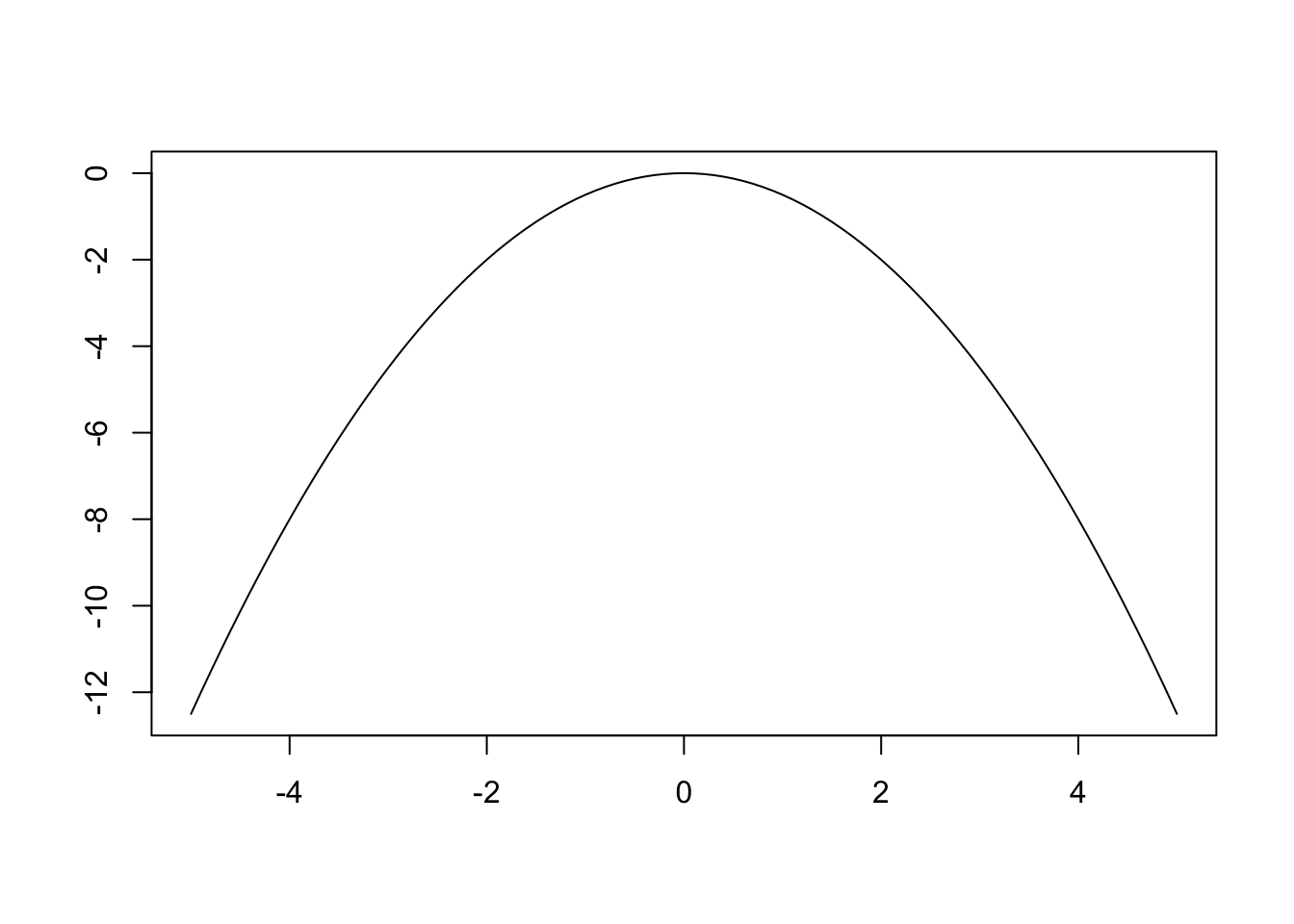
As you can see, this is a simple parabola. When we raise \(e\) to the power of \(-\frac{1}{2}x^2\) we get the following plot.
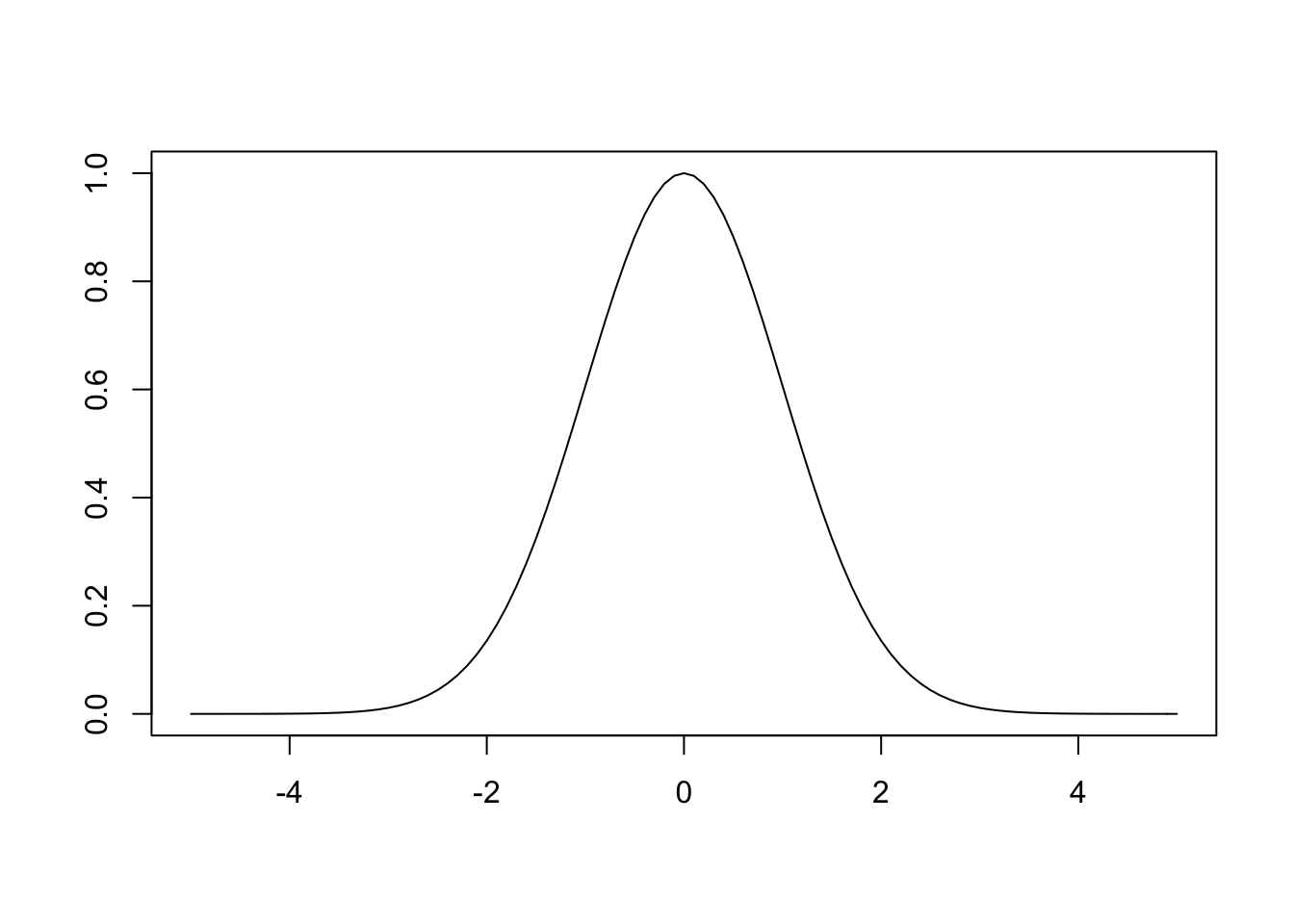
Taking the exponential of a negative parabola is what gives us the bell curve. However, there is still the issue that the area under the curve must be equal to 1 as the probability of all possible events must be equal to 1. As is, the area under the curve is \(2\pi\), so the constant \(\frac{1}{2\pi}\) is included.3 The \(e\) comes out of the derivation, but it is not critical, the math just works out more cleanly when \(e\) is used. The final thing to explain is the \(\frac{1}{2}\) in the exponent, which simply ensures that the variance is equal to 1. Now we can plot the entire function.
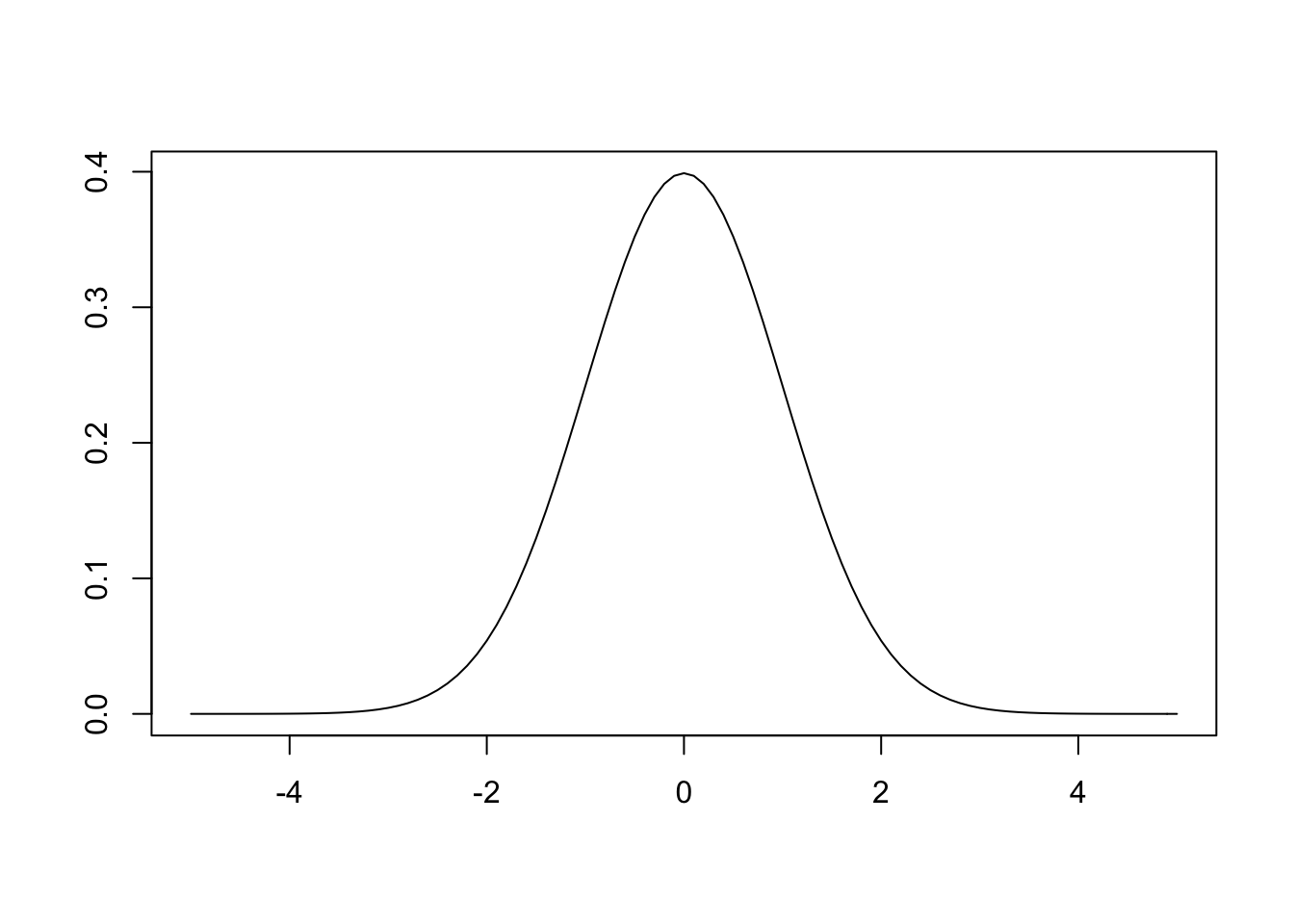
As expected, we get the standard normal curve. In order to generalize to any normal distribution we simply include the parameters μ and σ in (1.2).
\[\begin{equation} \LARGE \frac{1}{\sigma\sqrt{2\pi}}e^{-\frac{1}{2}{(\frac{x-\mu}{\sigma})}^2} \tag{1.2} \end{equation}\]
Notice that σ scales the constant, but that the real action happens in the exponent. The distribution’s highest point is shifted by μ, then divided by σ. Let’s take a closer look at what happens when we keep μ = 0 and set σ = 2. The exponent becomes \(\frac{-1}{2}{(\frac{x}{2})}^2\) which leads to the following plot.
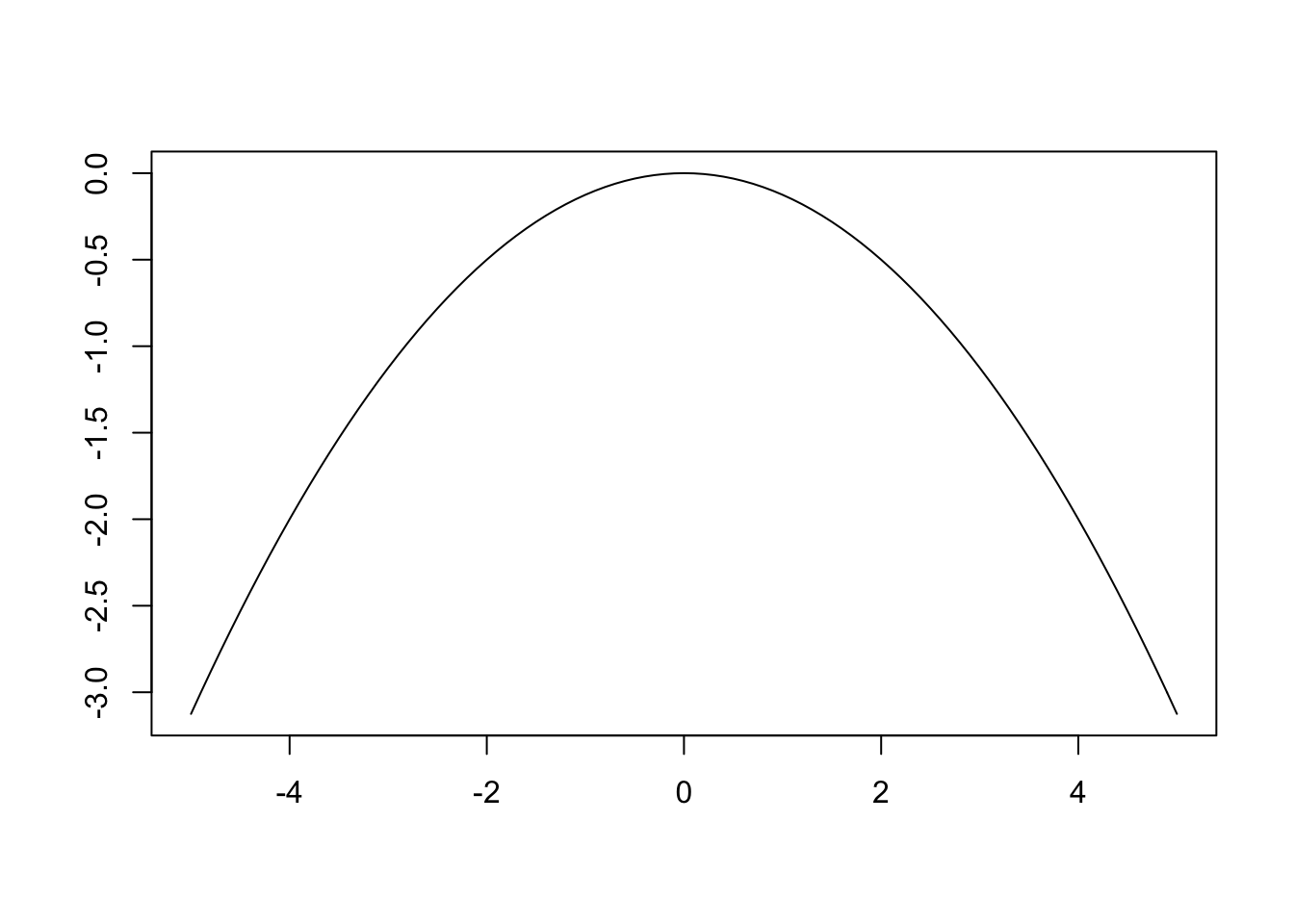
We observe a wider version of the parabola we saw previously. This makes sense as the exponent reduces to \(-\frac{x^2}{8}\) (as opposed to \(-\frac{x^2}{2}\) when σ = 1). The large denominator leads to values closer to 0 for the same values of x. This property is maintained (but flipped) after the value is plugged into \(e^{\frac{-1}{2}{(\frac{x}{2})}^2}\). For example, if x = 1 and σ = 1 the expression evaluates to 0.61 but when σ = 2 we get 0.88. Large values of σ lead to wider parabolas, which in turn lead to wider bell curves.
1.3.1 The Normal Distribution’s CDF
Now that we have explored the normal distribution’s probability density function, we can discuss the cumulative density function. As discussed above, when dealing with probability over continuous values we are primarily interested in probability over a range. For some purposes, it is convenient to think of a distribution in terms of total probability of an event occurring in the range of \(-\infty\) to x. This is where the cumulative distribution function comes in. For the standard normal distribution we get the cdf defined in (1.3) which is often denoted as \(\Phi\).
\[\begin{equation} \LARGE \frac{1}{\sqrt{2\pi}}\int_{-\infty}^x {e^{-t^2/2} dt} \tag{1.3} \end{equation}\]
We won’t work as hard to understand the cdf, instead we will just relate it to the pdf. Here is a plot of the standard normal cdf.
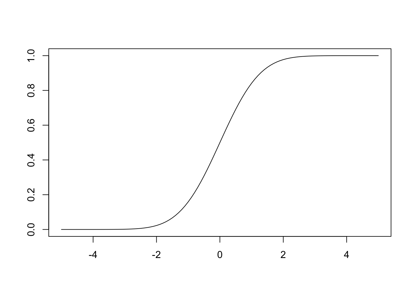
As described, the y axis shows cumulative probability so you will notice that the function is always increasing. Here is a widget to allow you to explore the normal pdf and cdf simultaneously. Click and drag the circles to change the value of x.
Hopefully you noticed that the cdf is simply expressing the area under the curve (i.e. the integral from \(-\infty\) to x) of the pdf. Let’s think about some specific values to help solidify the relationship here. With x = 0, we are at the mean of the standard normal, so values are equally likely to be less than or greater than x. This means that the cdf at x = 0 should be 0.5 as we have accumulated half of the available probability. We also know that at 2 σ above the mean (here that means x = 2) we should have accumulated about 97.5% of the total probability (think about constructing a 95% confidence interval, where we use z = 1.96). Go back to the widget and ensure that these intuitions are correct.
As aluded to above, confidence intervals are one way the normal cdf comes up. In fact, the cdf comes into play any time that you are interested in a probability range. For any two values you can simply subtract the cumulative densities to get the probability of a value occuring within that range. For example, if you are interested in the probability that a person’s IQ will fall within 1 σ of the mean, you can subtract the cdf value for x = -1 from the value for x = 1. Estimate this value using the widget.4
1.4 Working with the Normal Distribution in R
Values of the normal pdf and cdf can be easily accessed using R. As with all distributions, R provides functions for generating density (dnorm), cumulative density (pnorm) quantile (qnorm) and random (rnorm) values. By default, μ = 0 and σ = 1, but these values can be changes with the mean and sd arguments. Below are some examples showing how to use these functions.
## [1] 0.3989423# Useful for generating a normal plot, e.g.
x = seq(-3, 3, length.out=100)
y = dnorm(x)
plot(x, y, type='l')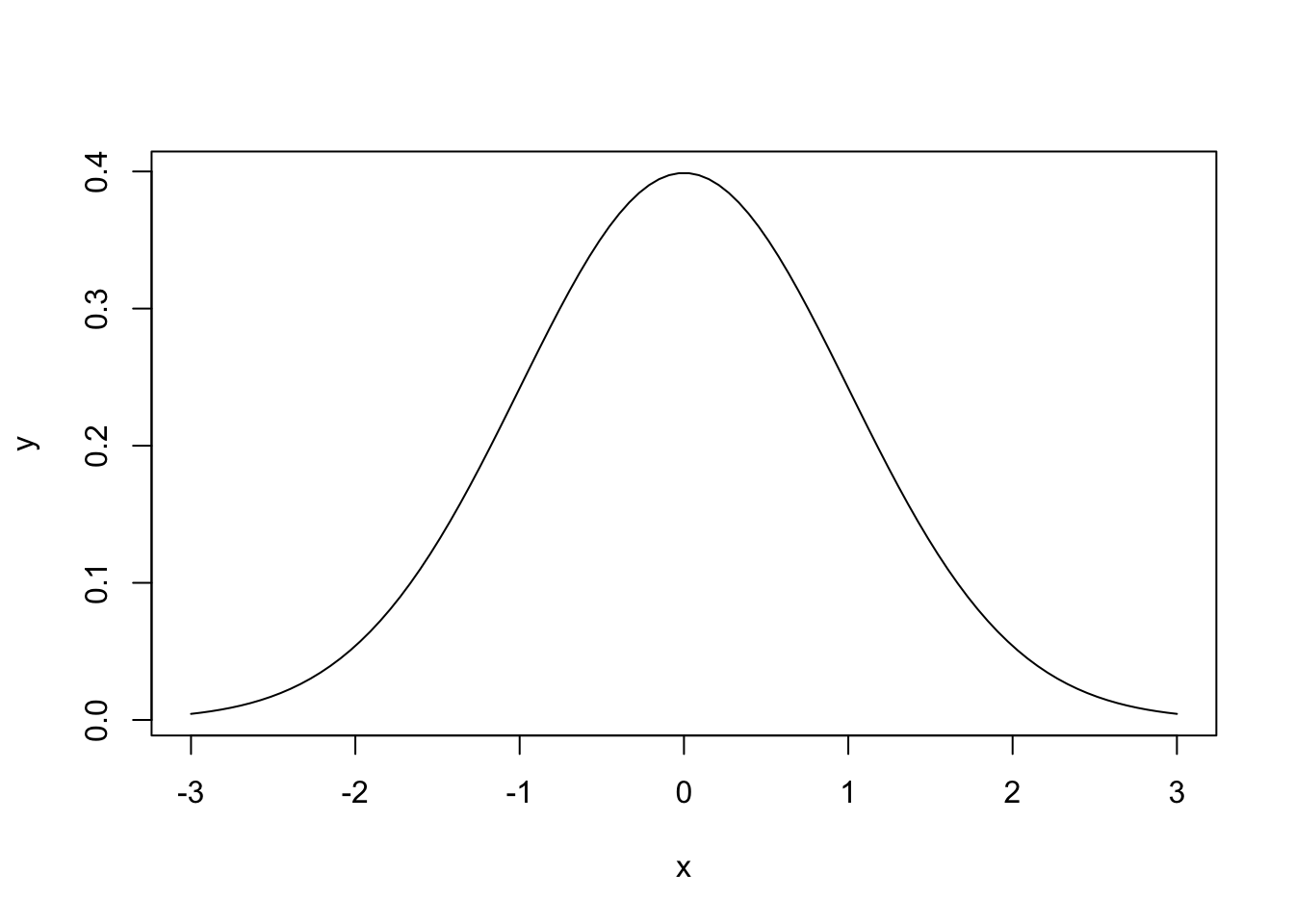
## [1] 0.5## [1] 0.9750021## [1] 0## [1] 1.959964Notice the relationship between qnorm and pnorm.
##  [1]  0.2816754 -2.8890201 -1.0463806  0.7035557  0.7382826 -1.1201823
##  [7]  0.3014865 -0.5977807 -0.3594820 -0.5061198
Note that if you go on for too long you end up with a uniform distribution. This is an artifact caused by the edges of the plot; performing the simulation with a larger number of frogs and for more steps will allow you to approximate the normal distribution more closely.↩
For discrete random variables a probability mass function (pmf) takes the place of the probability density function.↩
Note that when x = 0, you end up with \(\frac{1}{2\pi}e^0\) or simply \(\frac{1}{2\pi}\). The highest point in the standard normal curve comes from this constant.↩
As you may know, the true value is ~66%.↩