Chapter 9 General Knowledge

---

9.1 ggplot2

---

ggplot2 is a R package dedicated to data visualization. It can greatly improve the quality and aesthetics of your graphics, and will make you much more efficient in creating them.

ggplot2 allows to build almost any type of chart. The R graph gallery focuses on it so almost every section there starts with ggplot2 examples.

This page is dedicated to general ggplot2 tips that you can apply to any chart, like customizing a title, adding annotation, or using faceting. If you’re new to ggplot2, a good starting point is probably this online course.

9.1.1 Add Text Labels with ggplot2

This document is dedicated to text annotation with ggplot2. It provides several examples with reproducible code showing how to use function like geom_label and geom_text.

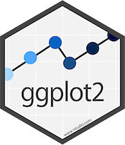
9.1.1.1 Adding Text with geom_text()

This example demonstrates how to use geom_text() to add text as markers. It works pretty much the same as geom_point(), but add text instead of circles. A few arguments must be provided:

• label: what text you want to display.
• nudge_x and nudge_y: shifts the text along X and Y axis.
• check_overlap tries to avoid text overlap. Note that a package called ggrepel extends this concept further.

# library
library(ggplot2)
 
# Keep 30 first rows in the mtcars natively available dataset
data=head(mtcars, 30)
 
# 1/ add text with geom_text, use nudge to nudge the text
ggplot(data, aes(x=wt, y=mpg)) +
  geom_point() + # Show dots
  geom_text(
    label=rownames(data), 
    nudge_x = 0.25, nudge_y = 0.25, 
    check_overlap = T
  )

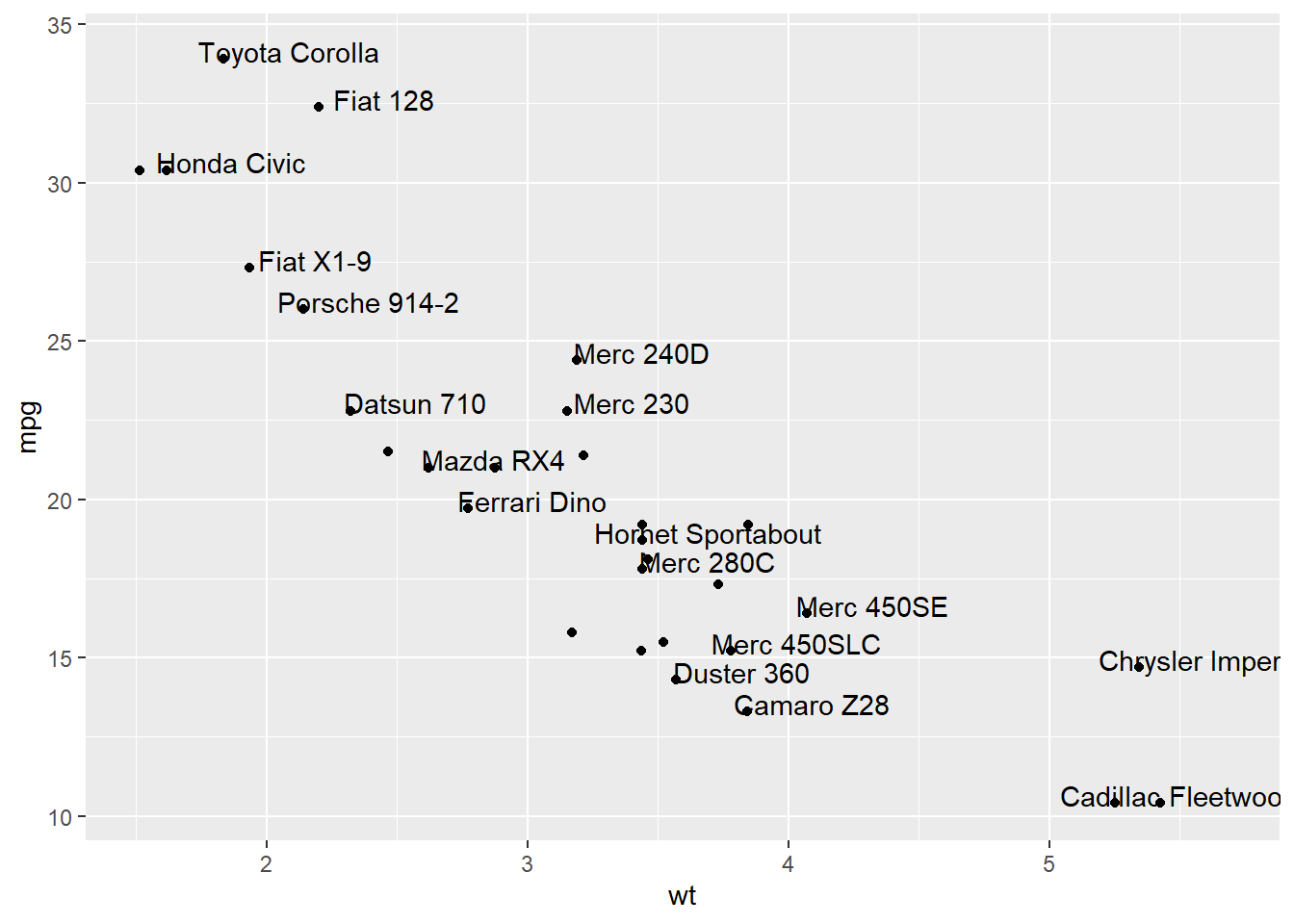
9.1.2 Add Labels with geom_label()

geom_label() works pretty much the same way as geom_text(). However, text is wrapped in a rectangle that you can customize (see next example).

# library
library(ggplot2)
 
# Keep 30 first rows in the mtcars natively available dataset
data=head(mtcars, 30)
 
# 1/ add text with geom_text, use nudge to nudge the text
ggplot(data, aes(x=wt, y=mpg)) +
  geom_point() + # Show dots
  geom_label(
    label=rownames(data), 
    nudge_x = 0.25, nudge_y = 0.25, 
    check_overlap = T
  )

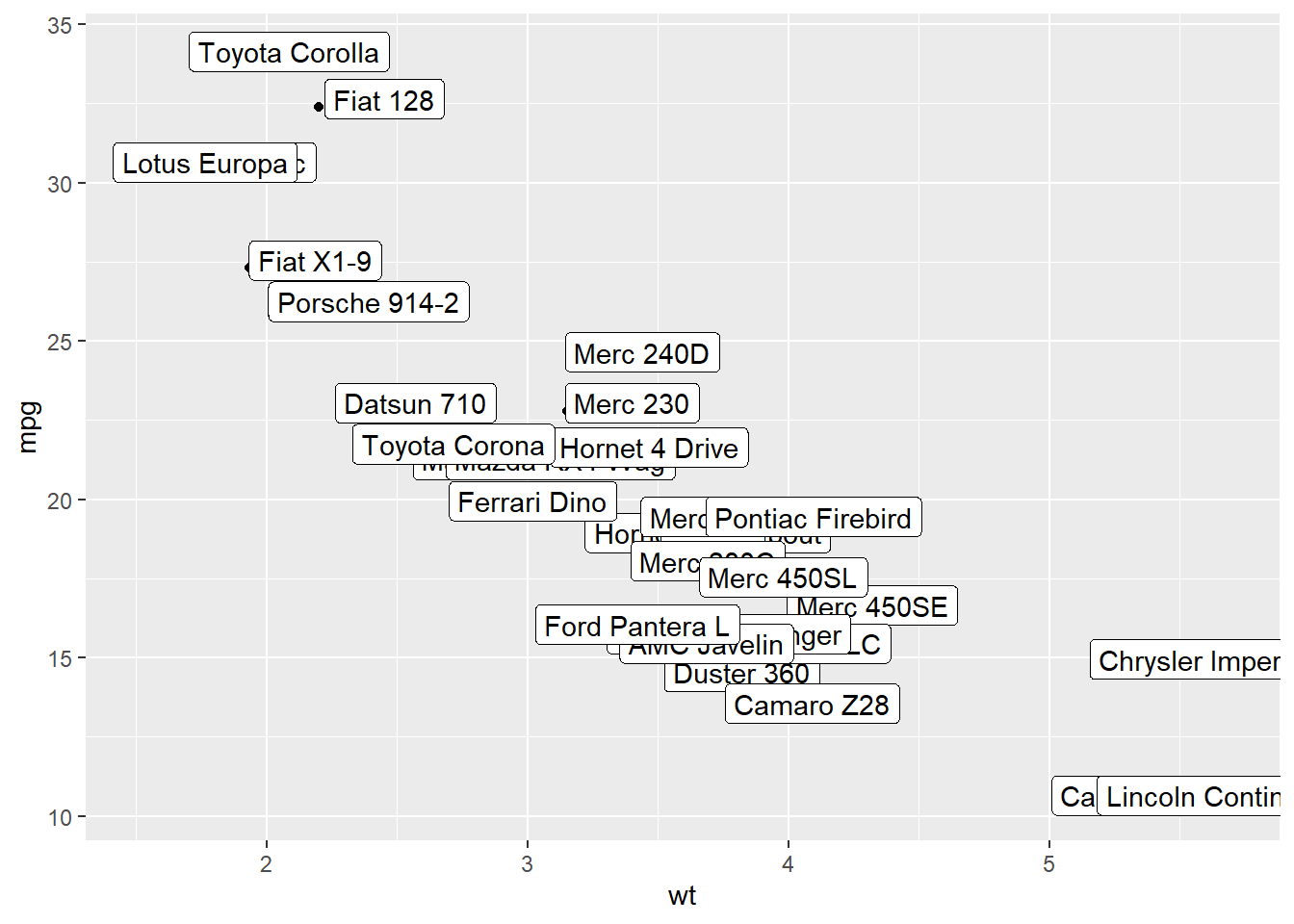
9.1.3 Add One Text Label Only

Of course, you don’t have to label all dots on the chart. You can also add a piece of text on a specific position. Since we’re here, note that you can custom the annotation of geom_label with label.padding, label.size, color and fill as described below:

# library
library(ggplot2)
 
# Keep 30 first rows in the mtcars natively available dataset
data=head(mtcars, 30)
 
# Add one annotation
ggplot(data, aes(x=wt, y=mpg)) +
  geom_point() + # Show dots
  geom_label(
    label="Look at this!", 
    x=4.1,
    y=20,
    label.padding = unit(0.55, "lines"), # Rectangle size around label
    label.size = 0.35,
    color = "black",
    fill="#69b3a2"
  )

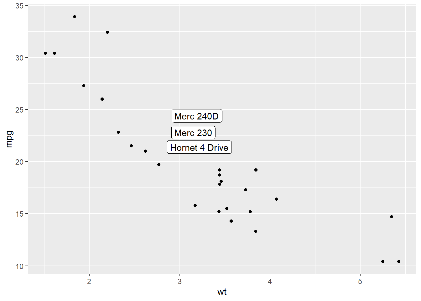
9.1.4 Add Labels for a Selection of Marker

Last but not least, you can also select a group of marker and annotate them only. Here, only car with mpg > 20 and wt > 3 are annotated thanks to a data filtering in the geom_label() call.

# library
library(ggplot2)
library(dplyr)
library(tibble)

# Keep 30 first rows in the mtcars natively available dataset
data=head(mtcars, 30)

# Change data rownames as a real column called 'carName'
data <- data %>%
  rownames_to_column(var="carName")
  
# Plot
ggplot(data, aes(x=wt, y=mpg)) +
  geom_point() + 
  geom_label( 
    data=data %>% filter(mpg>20 & wt>3), # Filter data first
    aes(label=carName)
  )

9.1.5 How to Annotate a Plot in ggplot2

Once your chart is done, annotating it is a crucial step to make it more insightful. This section will guide you through the best practices using R and ggplot2.

9.1.6 Adding text with geom_text() or geom_label()

Text is the most common kind of annotation. It allows to give more information on the most important part of the chart.

Using ggplot2, 2 main functions are available for that kind of annotation:

• geom_text: to add a simple piece of text.
• geom_label: to add a label: framed text.

Note that the annotate() function is a good alternative that can reduces the code length for simple cases.

# library
library(ggplot2)

# basic graph
p <- ggplot(mtcars, aes(x = wt, y = mpg)) + 
  geom_point()
 
# a data frame with all the annotation info
annotation <- data.frame(
   x = c(2,4.5),
   y = c(20,25),
   label = c("label 1", "label 2")
)

# Add text
p + geom_text(data=annotation, aes( x=x, y=y, label=label),                 
           color="orange", 
           size=7 , angle=45, fontface="bold" )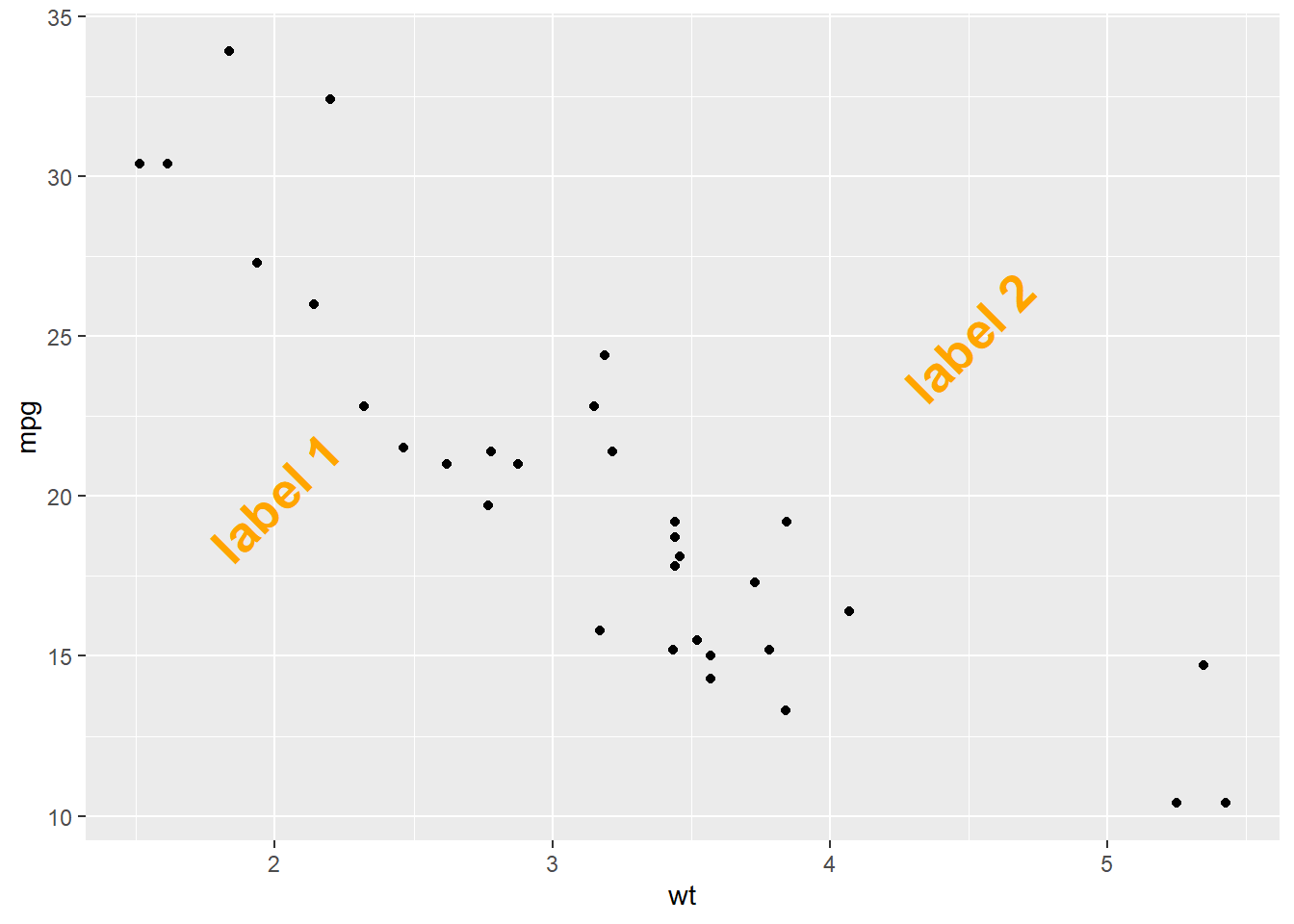

# Note: possible to shorten with annotate:
# p +
#  annotate("text", x = c(2,4.5), y = c(20,25), 
#           label = c("label 1", "label 2") , color="orange", 
#           size=7 , angle=45, fontface="bold")
# Right chart: using labels
p + geom_label(data=annotation, aes( x=x, y=y, label=label),                  
           color="orange", 
           size=7 , angle=45, fontface="bold" )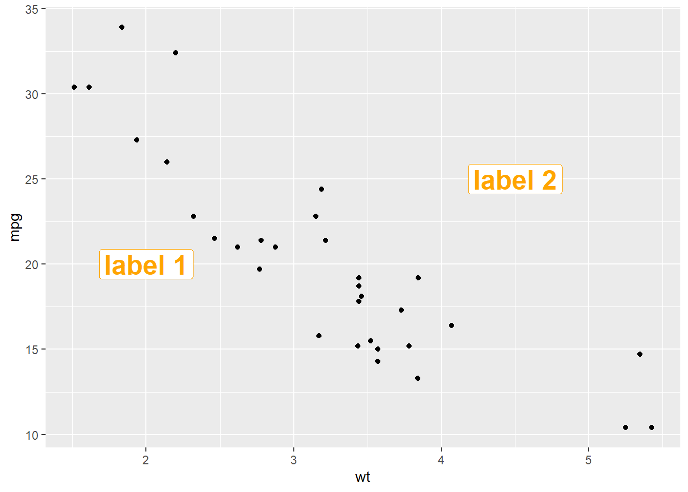

9.1.7 Add Shapes with annotate()

The annotate() function allows to add all kind of shape on a ggplot2 chart. The first argument will control what kind is used: rect or segment for rectangle, segment or arrow.

# Add rectangles
p + annotate("rect", xmin=c(2,4), xmax=c(3,5), ymin=c(20,10) , ymax=c(30,20), alpha=0.2, color="blue", fill="blue")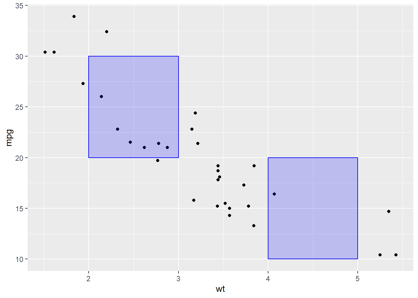

# Add segments
p + annotate("segment", x = 1, xend = 3, y = 25, yend = 15, colour = "purple", size=3, alpha=0.6)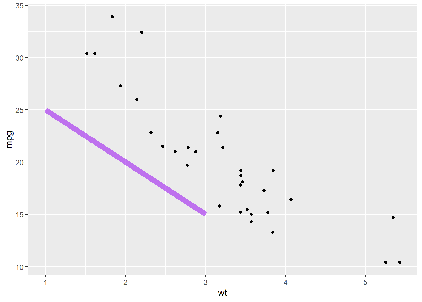

# Add arrow
p + annotate("segment", x = 2, xend = 4, y = 15, yend = 25, colour = "pink", size=3, alpha=0.6, arrow=arrow())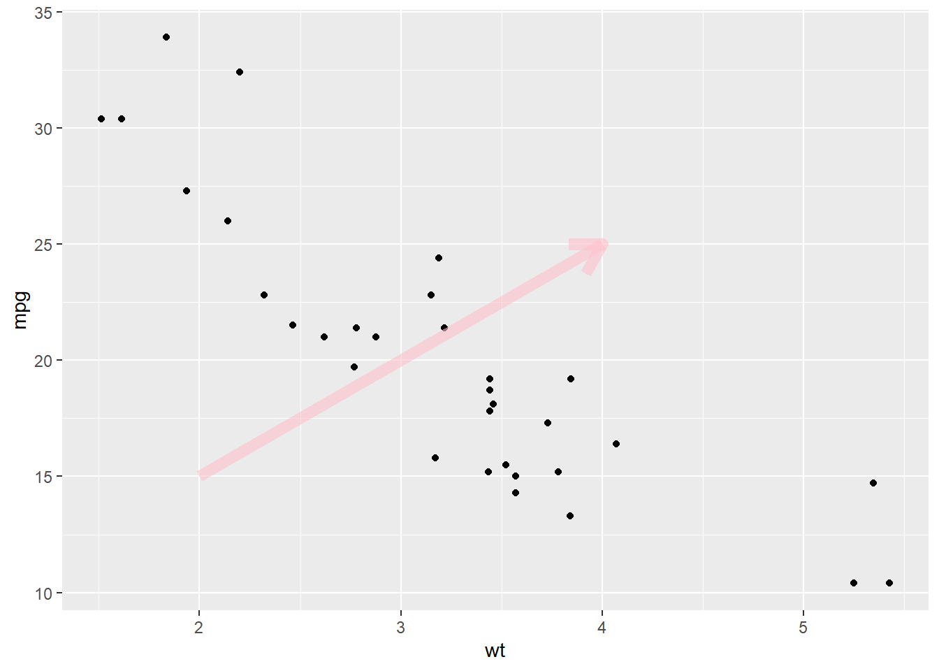

9.1.8 Add Ablines with geom_hline() and geom_vline()

An abline is a segment that goes from one chart extremity to the other. ggplot2 offers the geom_hline() and geom_vline() functions that are dedicated to it.

p + 
  # horizontal
  geom_hline(yintercept=25, color="orange", size=1) + 
  # vertical
  geom_vline(xintercept=3, color="orange", size=1)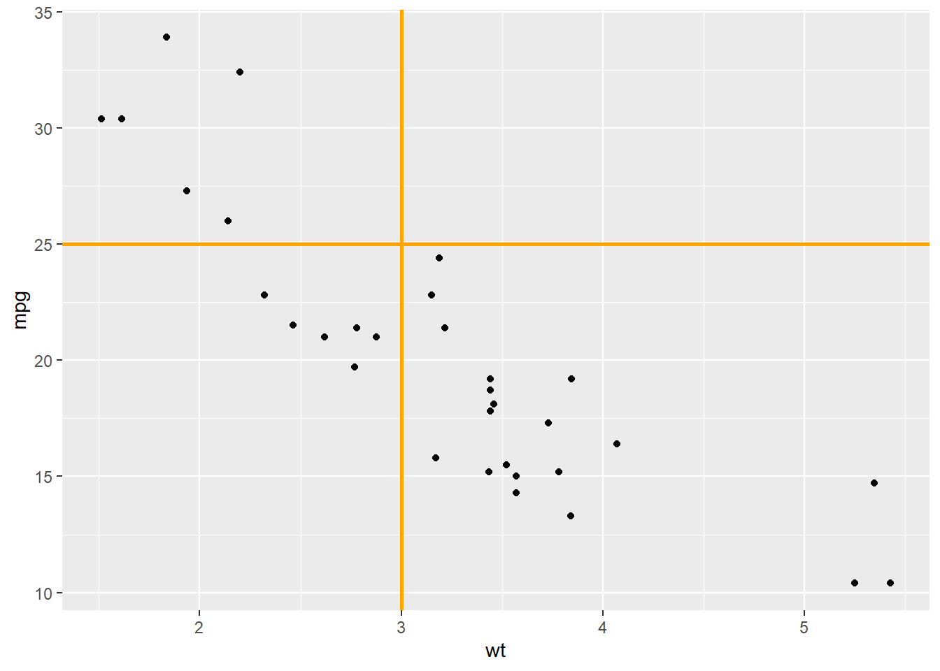

9.1.9 Add a Point and a Range with pointrange()

Last kind of annotation, add a dot and a segment directly with pointrange().

# Add point and range
p + annotate("pointrange", x = 3.5, y = 20, ymin = 12, ymax = 28,colour = "orange", size = 1.5, alpha=0.4)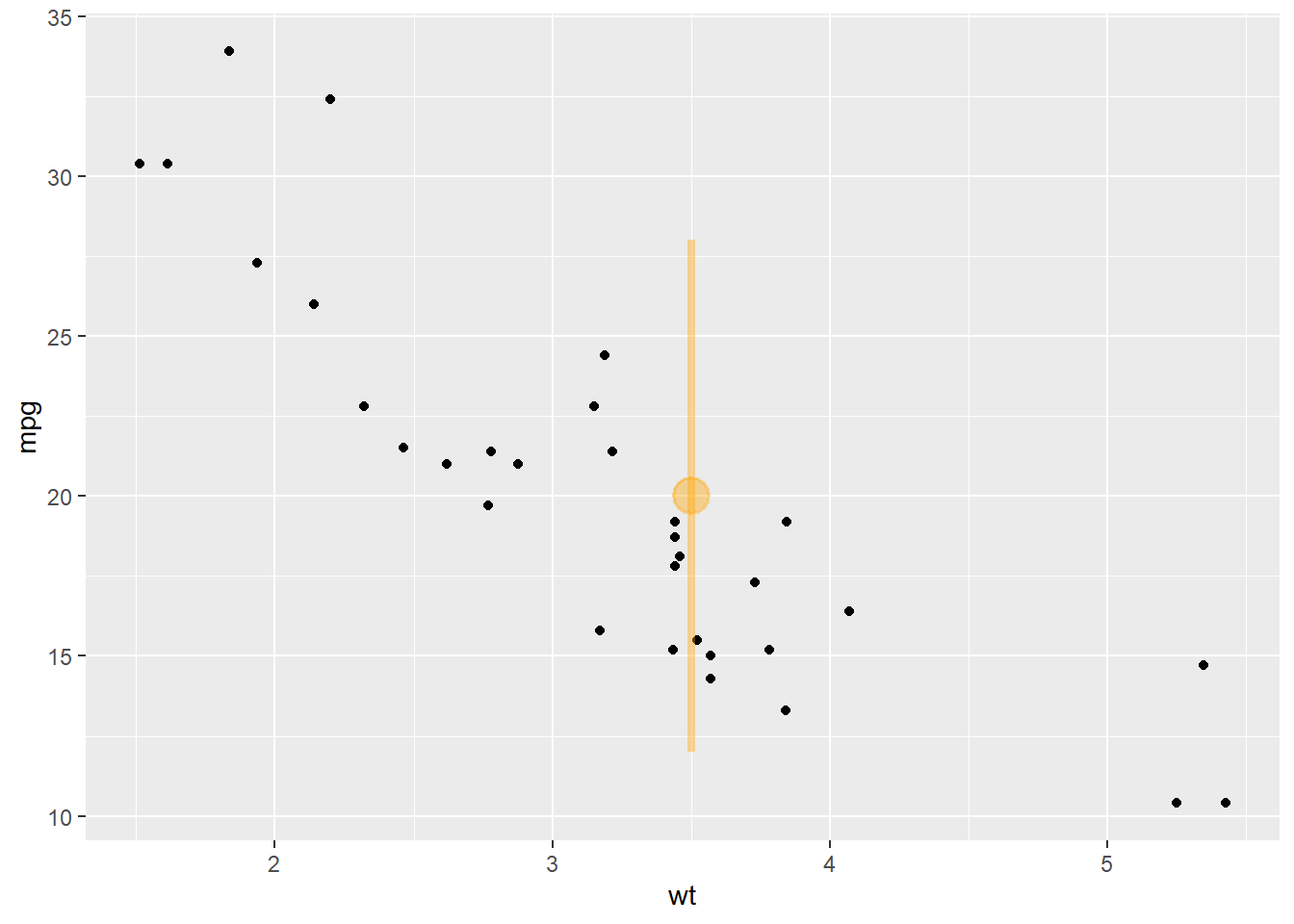

9.1.10 Marginal Plot

Marginal plots are not natively supported by ggplot2, but their realisation is straightforward thanks to theggExtra` library as illustrated in graph #277.

9.1.10.1 ggplot2 Scatterplot with Rug

This section demonstrates how to build a scatterplot with rug with R and ggplot2. Adding rug gives insight about variable distribution and is especially helpful when markers overlap.

9.1.10.2 Adding Rug with geom_rug()

A scatterplot displays the relationship between 2 numeric variables. You can easily add rug on X and Y axis thanks to the geom_rug() function to illustrate the distribution of dots.

Note you can as well add marginal plots to show these distributions.

# library
library(ggplot2)

# Iris dataset
head(iris)

##   Sepal.Length Sepal.Width Petal.Length Petal.Width Species
## 1          5.1         3.5          1.4         0.2  setosa
## 2          4.9         3.0          1.4         0.2  setosa
## 3          4.7         3.2          1.3         0.2  setosa
## 4          4.6         3.1          1.5         0.2  setosa
## 5          5.0         3.6          1.4         0.2  setosa
## 6          5.4         3.9          1.7         0.4  setosa

# plot
ggplot(data=iris, aes(x=Sepal.Length, Petal.Length)) +
  geom_point() +
  geom_rug(col="steelblue",alpha=0.1, size=1.5)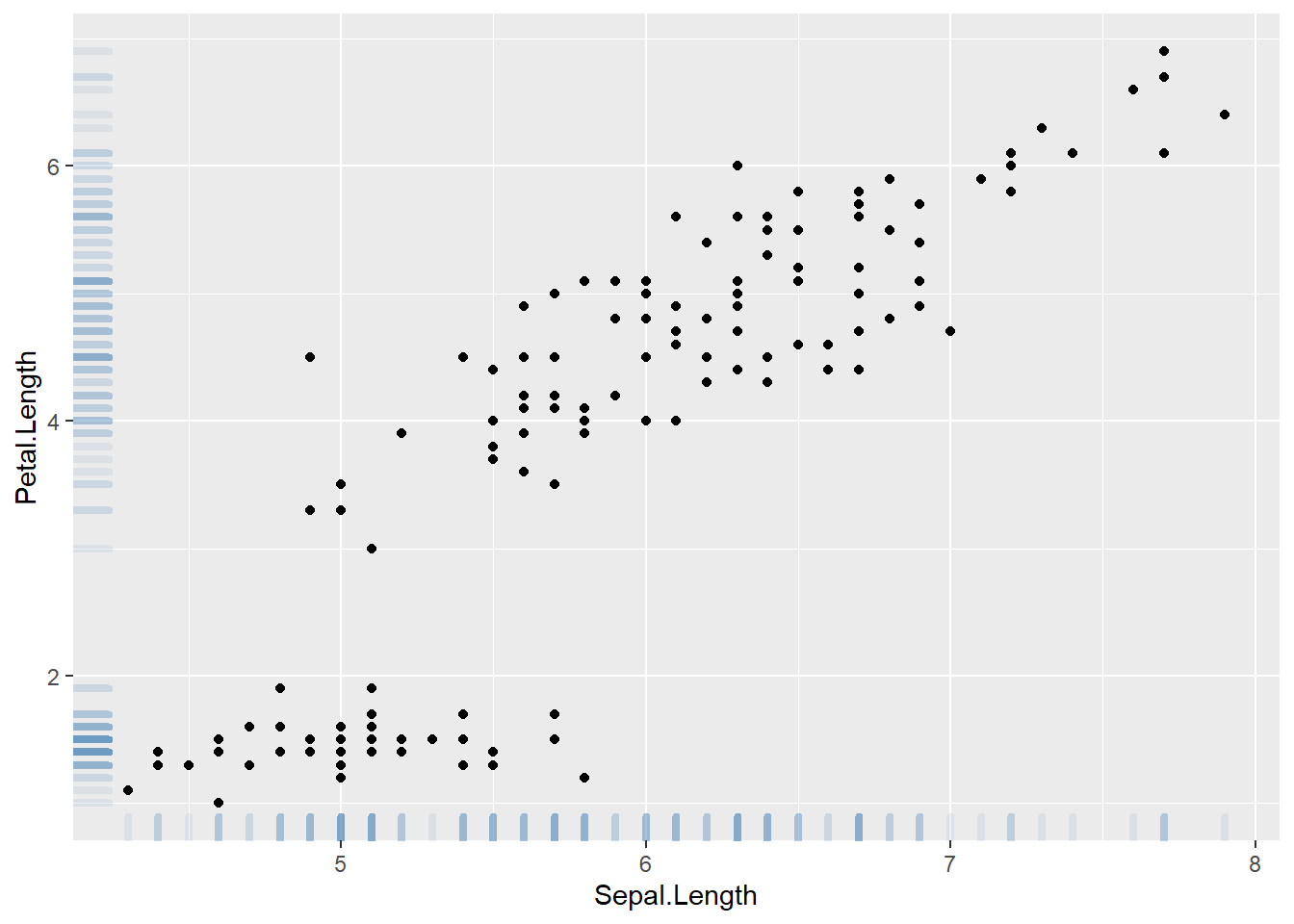

9.1.11 Marginal Distribution with ggplot2 and ggExtra

This section explains how to add marginal distributions to the X and Y axis of a ggplot2 scatterplot. It can be done using histogram, boxplot or density plot using the ggExtra library.

9.1.11.1 Basic use of ggMarginal()

Here are 3 examples of marginal distribution added on X and Y axis of a scatterplot. The ggExtra library makes it a breeze thanks to the ggMarginal() function. Three main types of distribution are available: histogram, density and boxplot.

# library
library(ggplot2)
library(ggExtra)
 
# The mtcars dataset is proposed in R
head(mtcars)

##                    mpg cyl disp  hp drat    wt  qsec vs am gear carb
## Mazda RX4         21.0   6  160 110 3.90 2.620 16.46  0  1    4    4
## Mazda RX4 Wag     21.0   6  160 110 3.90 2.875 17.02  0  1    4    4
## Datsun 710        22.8   4  108  93 3.85 2.320 18.61  1  1    4    1
## Hornet 4 Drive    21.4   6  258 110 3.08 3.215 19.44  1  0    3    1
## Hornet Sportabout 18.7   8  360 175 3.15 3.440 17.02  0  0    3    2
## Valiant           18.1   6  225 105 2.76 3.460 20.22  1  0    3    1

# classic plot :
p <- ggplot(mtcars, aes(x=wt, y=mpg, color=cyl, size=cyl)) +
      geom_point() +
      theme(legend.position="none")
 
# with marginal histogram
p1 <- ggMarginal(p, type="histogram")
 
# marginal density
p2 <- ggMarginal(p, type="density")
 
# marginal boxplot
p3 <- ggMarginal(p, type="boxplot")

p1
p2
p3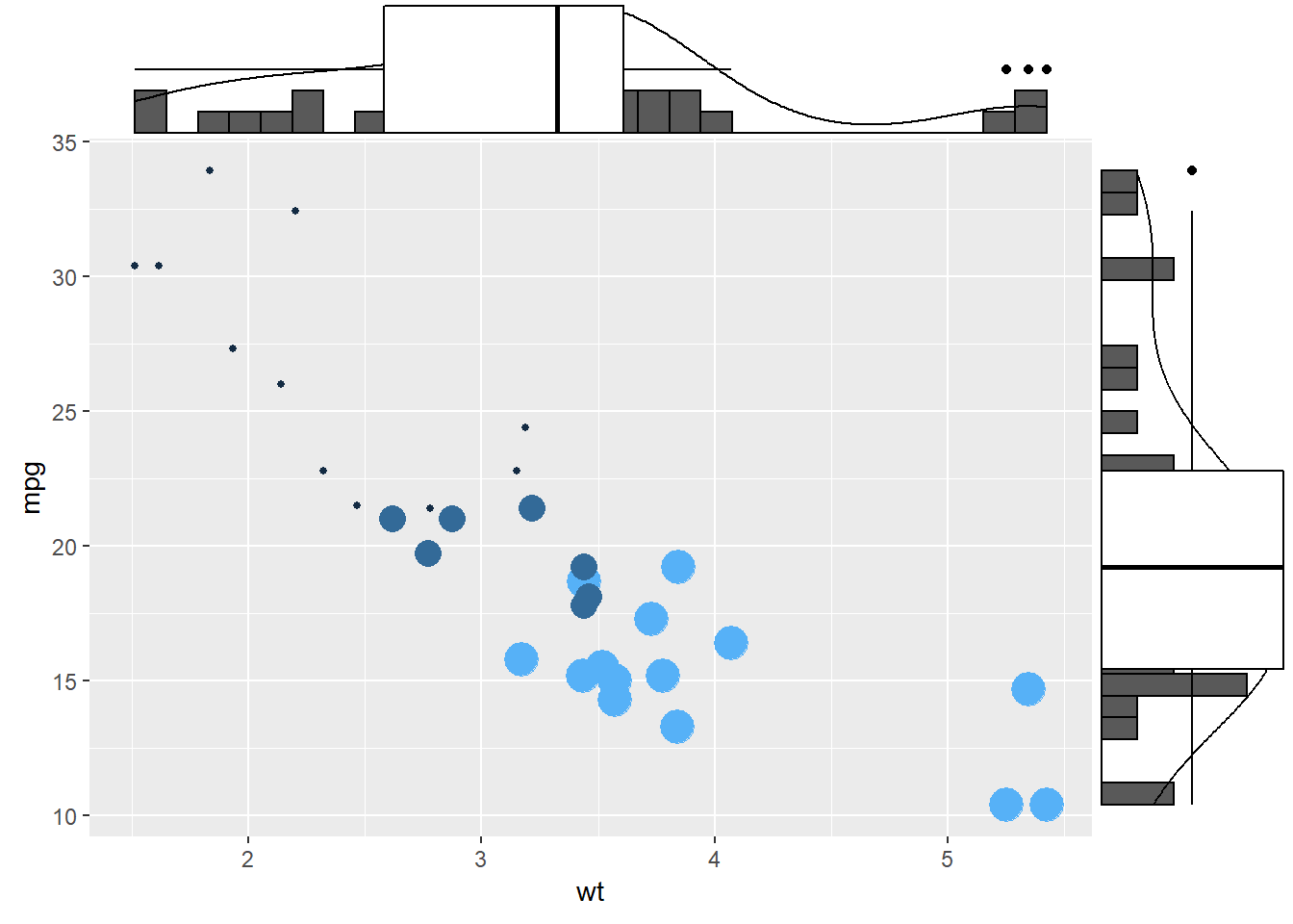

9.1.12 More Customization

Three additional examples to show possible customization:

• Change marginal plot size with size.
• Custom marginal plot appearance with all usual parameters.
• Show only one marginal plot with margins = 'x' or margins = 'y'.

# library
library(ggplot2)
library(ggExtra)
 
# The mtcars dataset is proposed in R
head(mtcars)

##                    mpg cyl disp  hp drat    wt  qsec vs am gear carb
## Mazda RX4         21.0   6  160 110 3.90 2.620 16.46  0  1    4    4
## Mazda RX4 Wag     21.0   6  160 110 3.90 2.875 17.02  0  1    4    4
## Datsun 710        22.8   4  108  93 3.85 2.320 18.61  1  1    4    1
## Hornet 4 Drive    21.4   6  258 110 3.08 3.215 19.44  1  0    3    1
## Hornet Sportabout 18.7   8  360 175 3.15 3.440 17.02  0  0    3    2
## Valiant           18.1   6  225 105 2.76 3.460 20.22  1  0    3    1

# classic plot :
p <- ggplot(mtcars, aes(x=wt, y=mpg, color=cyl, size=cyl)) +
      geom_point() +
      theme(legend.position="none")
 
# Set relative size of marginal plots (main plot 10x bigger than marginals)
p1 <- ggMarginal(p, type="histogram", size=10)
 
# Custom marginal plots:
p2 <- ggMarginal(p, type="histogram", fill = "slateblue", xparams = list(  bins=10))
 
# Show only marginal plot for x axis
p3 <- ggMarginal(p, margins = 'x', color="purple", size=4)

p1
p2
p3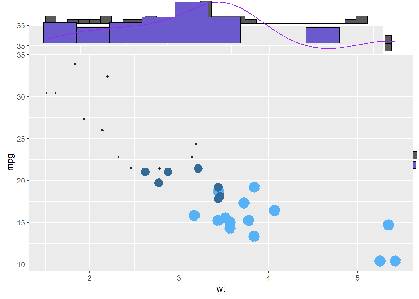

9.1.13 ggplot2 Chart Appearance

The theme() function of ggplot2 allows to customize the chart appearance. It controls 3 main types of components:

• Axis: controls the title, label, line and ticks.
• Background: controls the background color and the major and minor grid lines.
• Legend: controls position, text, symbols and more.

9.1.13.1 Axis Manipulation with R and ggplot2

This section describes all the available options to customize chart axis with R and ggplot2. It shows how to control the axis itself, its label, title, position and more.

9.1.13.2 Default ggplot2 Axis

Let’s start with a very basic ggplot2 scatterplot. The axis usually looks very good with default option as you can see here.

Basically two main functions will allow to customize it:

• theme() to change the axis appearance.
• scale_x_ and scale_y_ to change the axis type.

Let’s see how to use them

# Load ggplot2
library(ggplot2)

# Very basic chart
basic <- ggplot( mtcars , aes(x=mpg, y=wt)) + 
  geom_point()
basic

9.1.14 Set Axis Title and Limits with xlab() and xlim()

Two basic options that are used in almost every charts are xlab() and xlim() to control the axis title and the axis limits respectively.

Note: it’s possible to specify only the lower or upper bound of a limit. For instance, try xlim(0,NA)

basic+
    xlab("mpg value") + 
    xlim(0,50)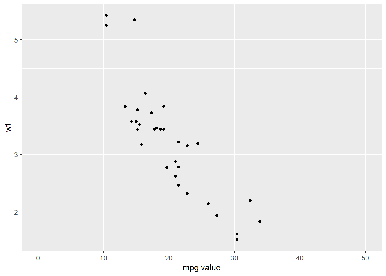

9.1.15 Customize Axis Title Appearance: axis.title

The theme() function allows to customize all parts of the ggplot2 chart. The axis.title. controls the axis title appearance. Since it is text, features are wrapped in a element_text() function. The code below shows how to change the most common features:

# Left -> both axis are modified
basic + theme(axis.title = element_text( angle = 90, color="red", size=15, face=3)) # face = title location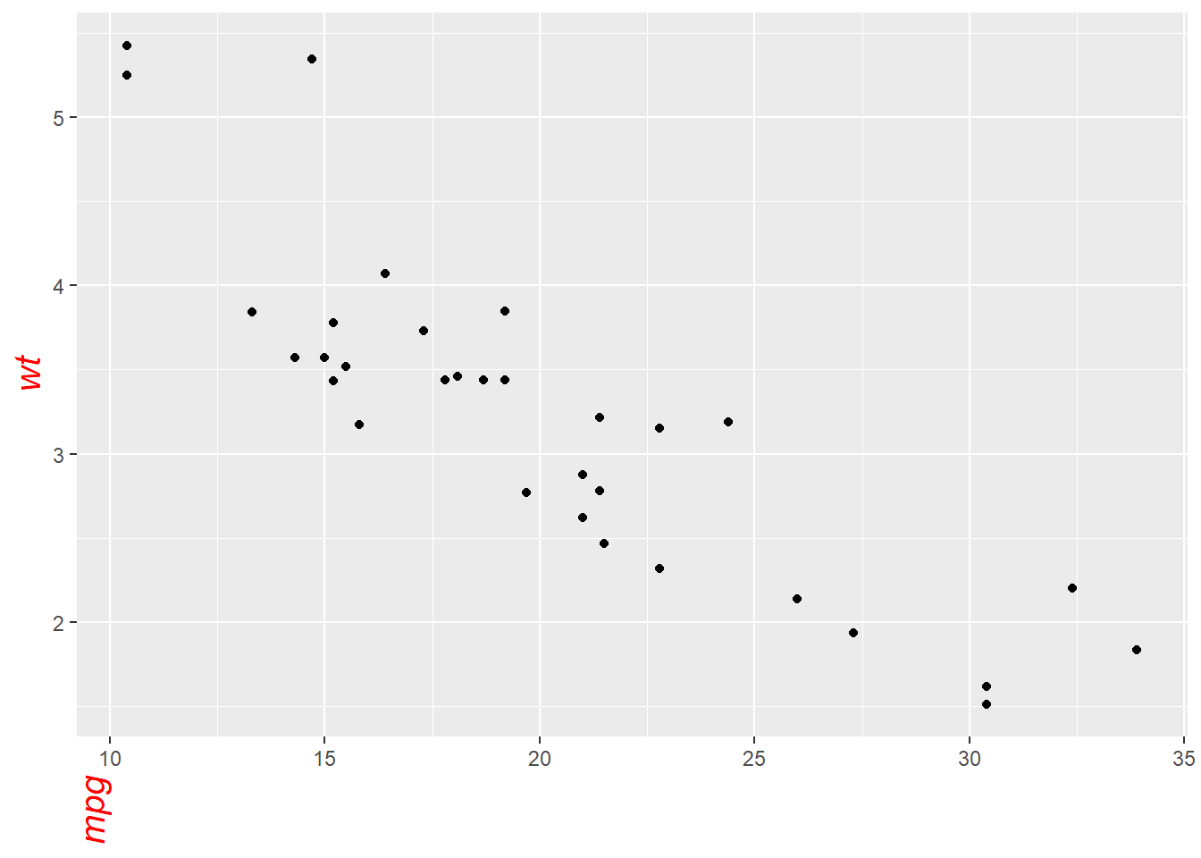

# Right -> only the x axis is modified
basic + theme(axis.title.x = element_text( angle = 90, color="red", size=15, face=3))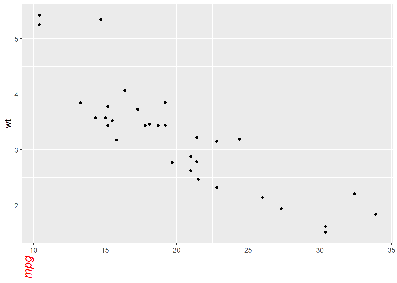

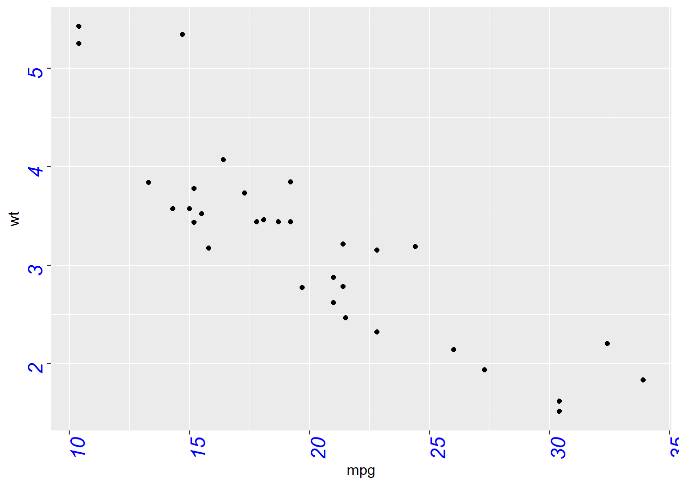
9.1.16 Customize Axis Labels: axis.text

Using pretty much the same process, the axis.text() function allows to control text label features. Once more, using axis.text.x() would modify the x axis only.

basic + 
  theme(axis.text = element_text( 
    angle = 90, 
    color="blue", 
    size=15, 
    face=3)
  )

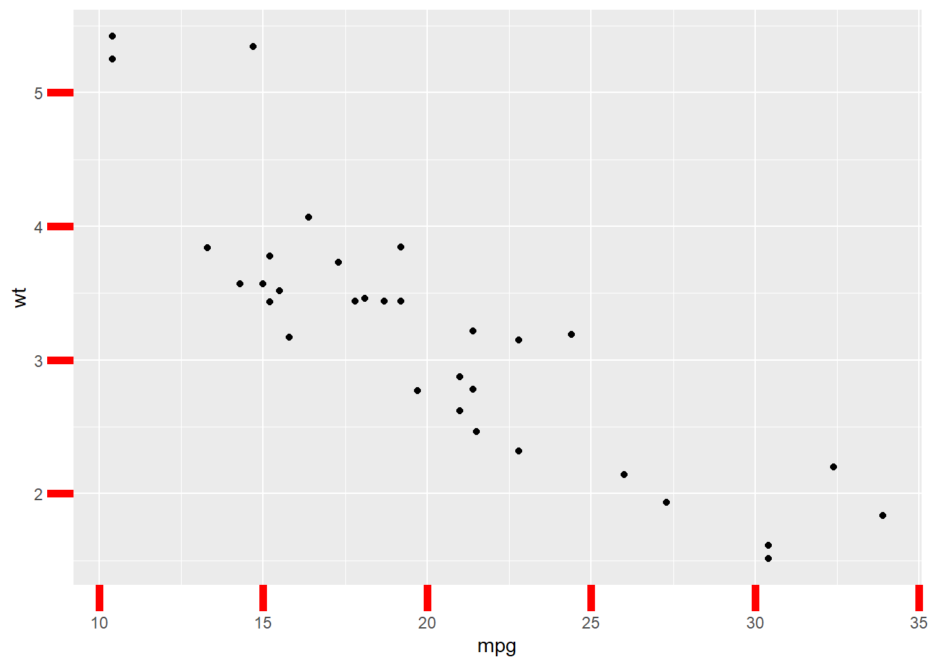
9.1.17 Customize Axis Ticks and Axis Line with axis.ticks() and axis.line()

The axis.ticks() function controls the ticks appearance. axis.line() controles the axis line. Both of them are lines, so options are wrapped in a element_line() statement.

linetype controls the type of line in use, see the ggplot2 section for more.

# chart 1: ticks
basic + theme(
   axis.ticks = element_line(size = 2, color="red") , 
   axis.ticks.length = unit(.5, "cm")
)

# chart 2: axis lines
basic + theme(axis.line = element_line(size = 3, colour = "green", linetype=2))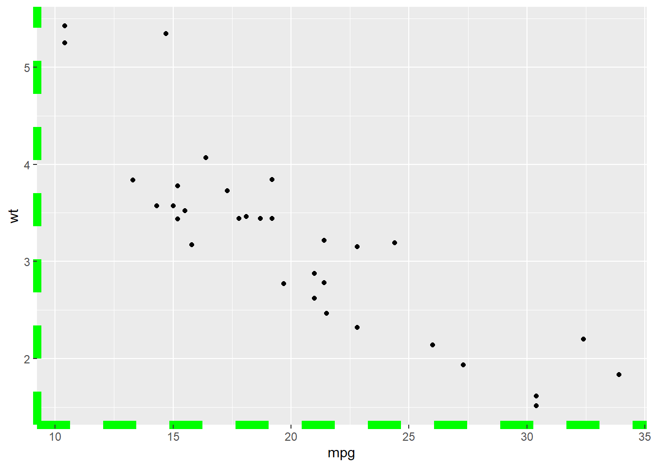

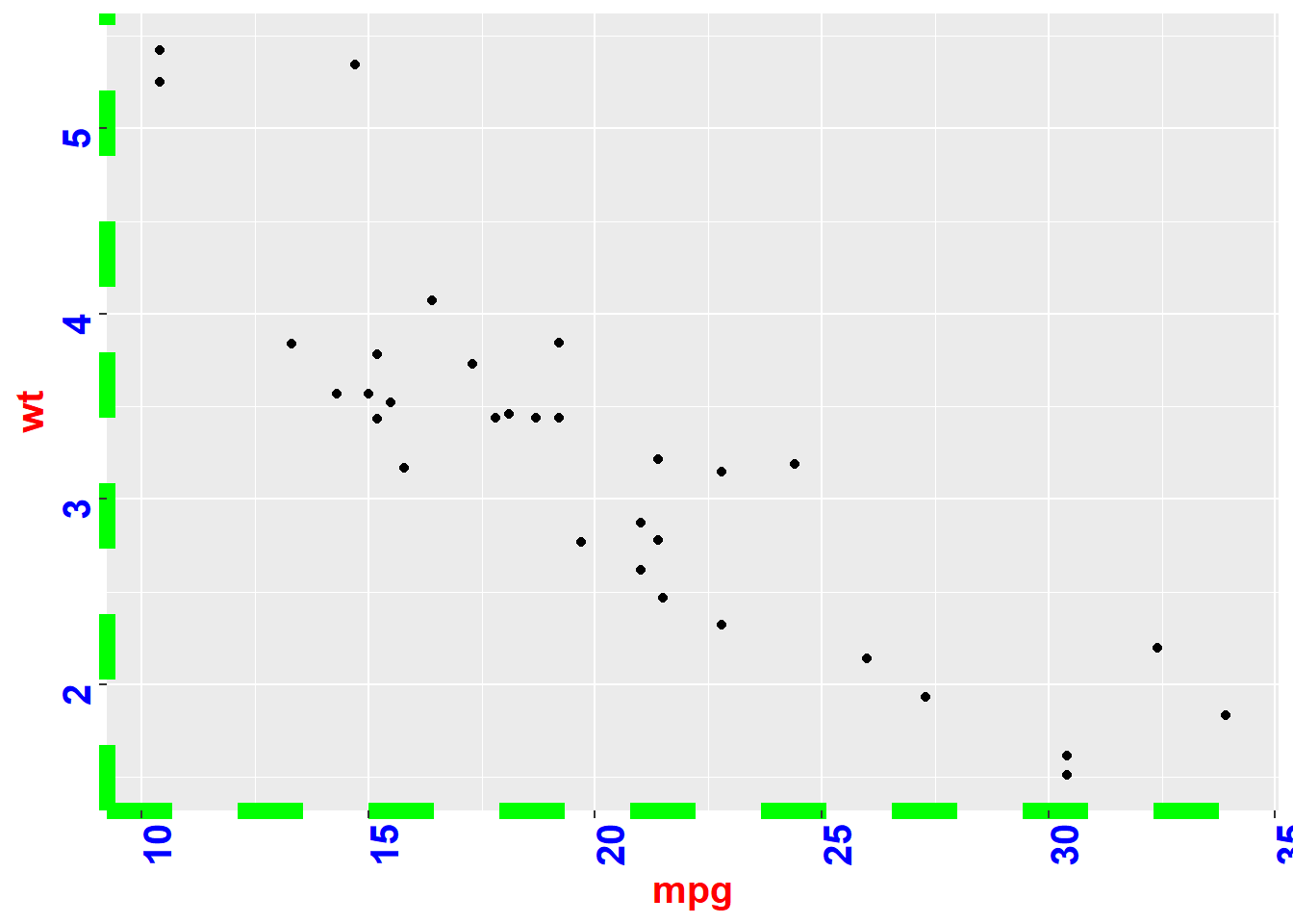
# chart 3: combination
ggplot( mtcars , aes(x=mpg, y=wt)) + geom_point() +
    theme(
        axis.title = element_text( color="red", size=15, face=2),
        axis.line = element_line(size = 3, colour = "green", linetype=2),
        axis.text = element_text( angle = 90, color="blue", size=15, face=2)
        )

9.1.18 Background Manipulation with R and ggplot2

This section describes all the available options to customize chart background with R and ggplot2. It shows how to control the background color and the minor and major gridlines.

9.1.18.1 Default ggplot2 Background

Let’s start with a very basic ggplot2 scatterplot. By default, ggplot2 offers a grey background with white major and minor gridlines.

It is possible to change that thanks to the theme() function. Keep reading to learn how!

# Load ggplot2
library(ggplot2)

# Very basic chart
basic <- ggplot( mtcars , aes(x=mpg, y=wt)) +
  geom_point()
basic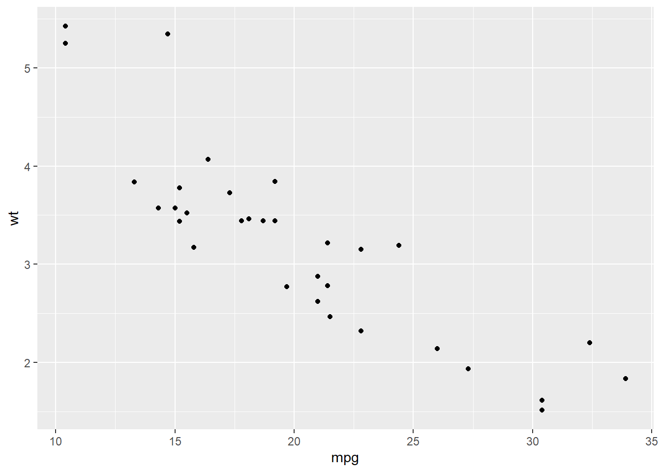

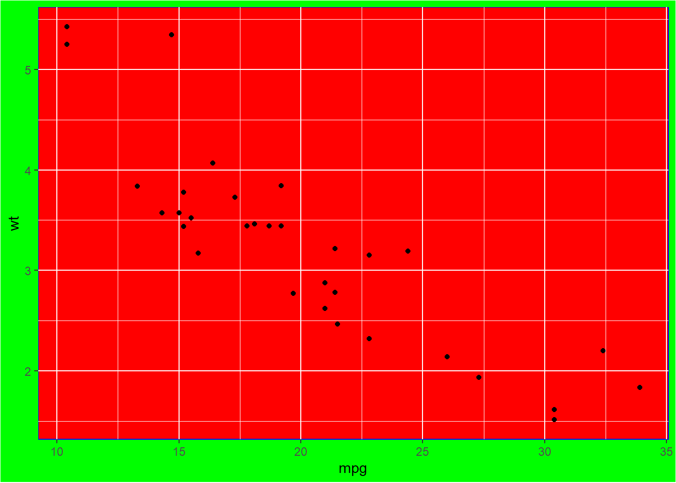
9.1.19 Background Color: plot.background and panel.background

Two options of the theme() functions are available to control the map background color. plot_background controls the color of the whole chart. panel.background controls the part between the axis.

Both are rectangles, with features specified through an element_rect() function.

basic + theme(
    plot.background = element_rect(fill = "green"), 
    panel.background = element_rect(fill = "red", colour="blue")
    )

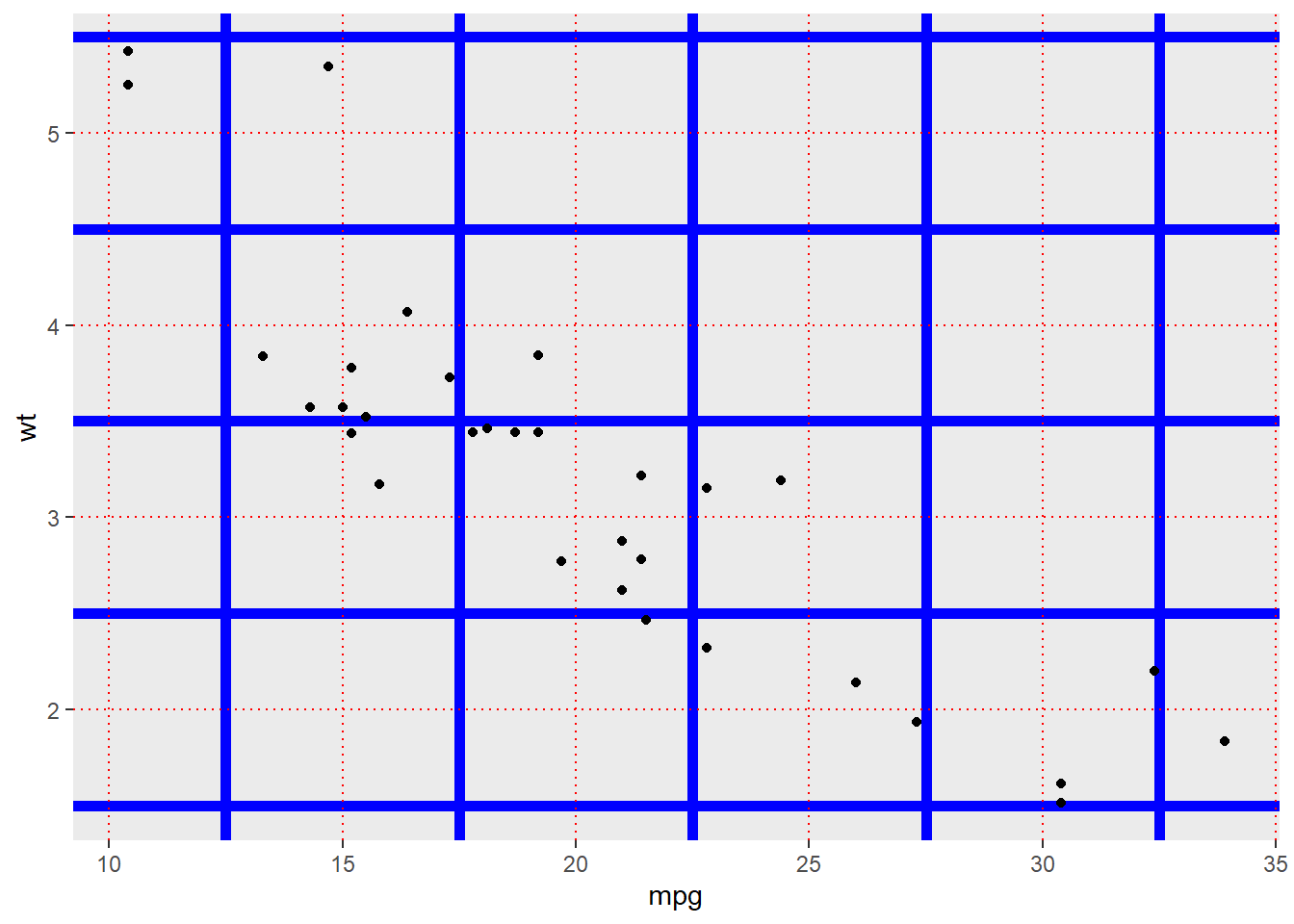
9.1.20 Customize the Grid: panel.grid.major and panel.grid.minor

Two main types of grid exist with ggplot2: major and minor. They are controlled thanks to the panel.grid.major and panel.grid.minor options.

Once more, you can add the options .y or .x at the end of the function name to control one orientation only.

Features are wrapped in an element_line() function. Specifying element_blanck() will simply removing the grid.

# Modify for both axis
basic + theme(
    panel.grid.major = element_line(colour = "red", linetype = "dotted"),
    panel.grid.minor = element_line(colour = "blue", size = 2)
    )

# Modify y axis only (remove)
basic + theme(
    panel.grid.major.y = element_blank(),
    panel.grid.minor.y = element_blank()
)

9.1.21 Building a Nice Legend with R and ggplot2

This section describes all the available options to customize the chart legend with R and ggplot2. It shows how to control the title, text, location, symbols and more.

9.1.21.1 Default Legend with ggplot2

By default, ggplot2 will automatically build a legend on your chart as soon as a shape feature is mapped to a variable in aes() part of the ggplot() call. So if you use color, shape or alpha, a legend will be available.

Here is an example based on the mtcars dataset. This section is gonna show how to use the theme() function to apply all type of customization on this default legend.

Note: this post is strongly inspired by the doc you get typing ggplot2::theme, give it a go!

# Load ggplot2
library(ggplot2)

# Very basic chart
basic <- ggplot(mtcars, aes(wt, mpg, colour = factor(cyl), shape = factor(vs) )) +
       geom_point()
basic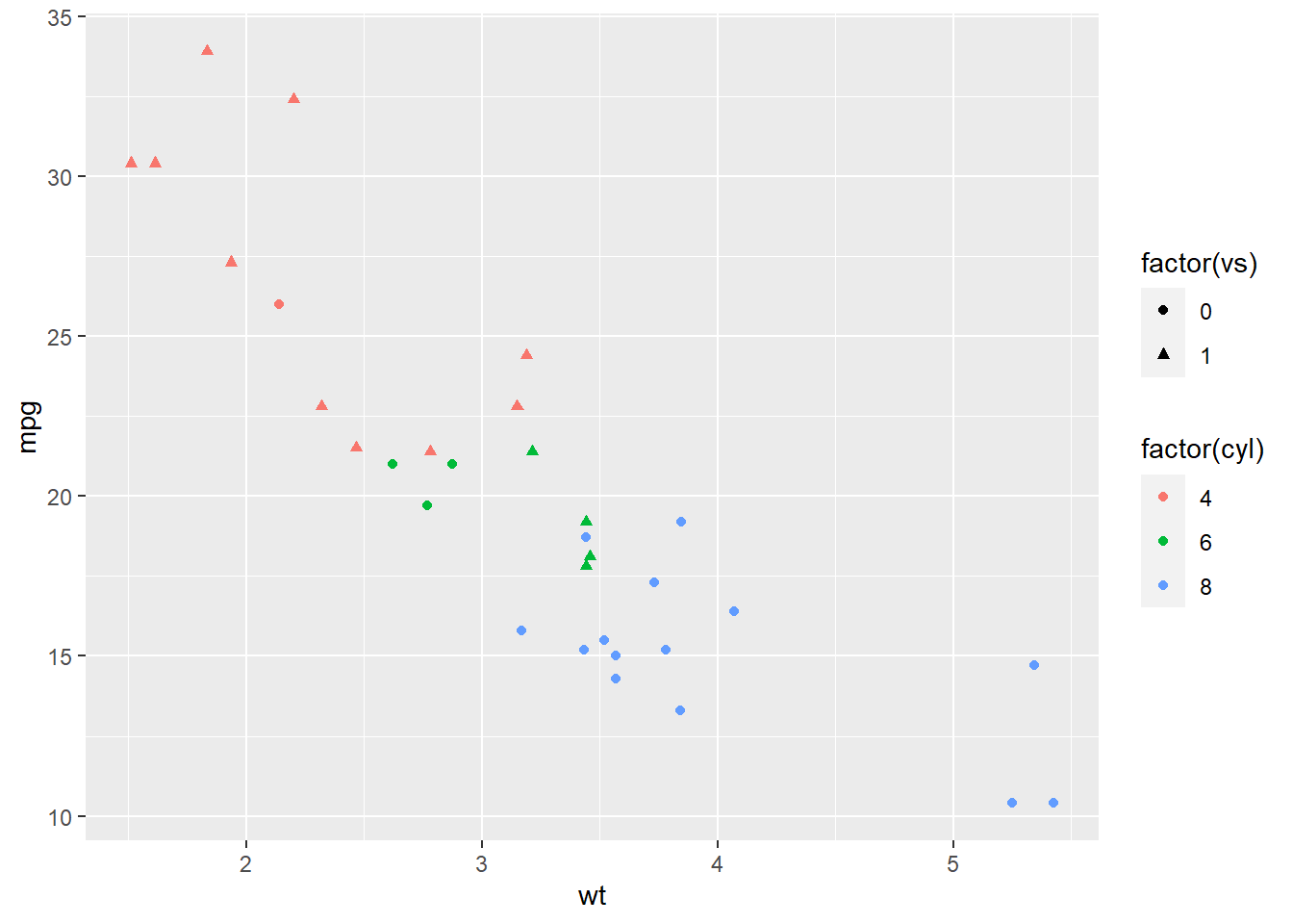

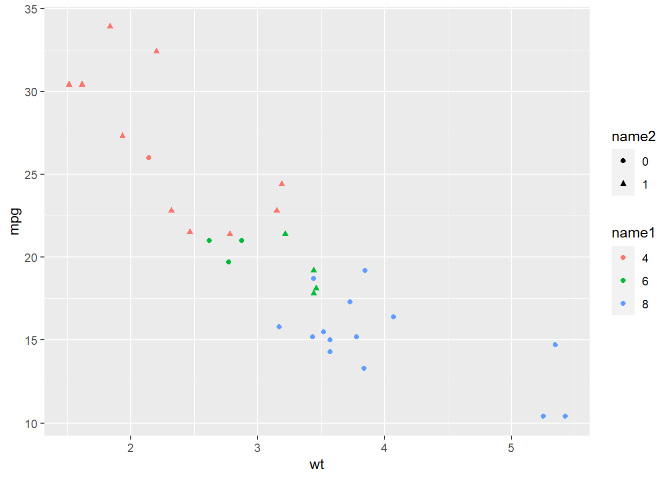
9.1.22 Change Legend Title with labs()

The labs() function allows to change the legend titles. You can specify one title per section of the legend, i.e. per aesthetics in use in the chart.

basic+
  labs(
         colour = "name1",
         shape = "name2"
        )

9.1.23 Get Rid of the Legend: guides() and theme()

It is possible to remove a specific part or the whole legend thanks to the theme() and the guides() function. See code below:

# Left -> get rid of one part of the legend
basic + guides(shape=FALSE)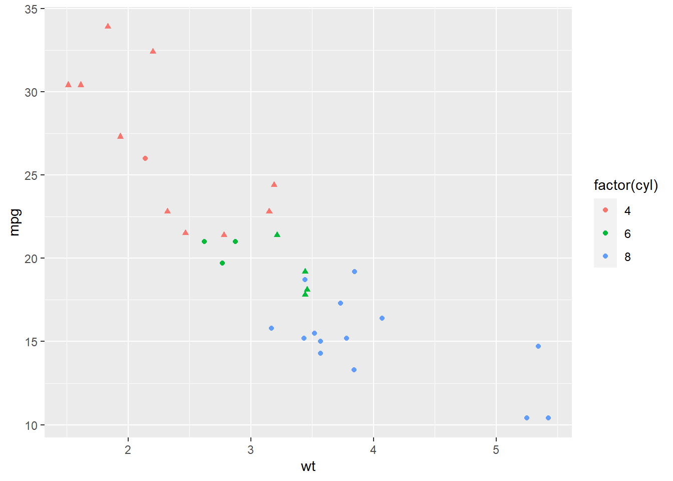

# Right -> only the x axis is modified
basic + theme(legend.position = "none")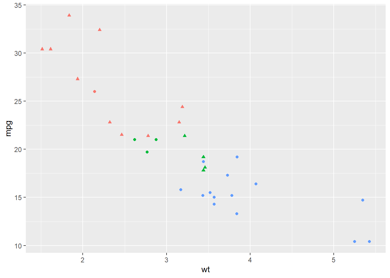

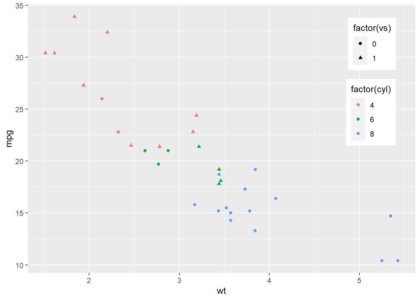
9.1.24 Control Legend Position with legend.position

You can place the legend literally anywhere.

To put it around the chart, use the legend.position option and specify top, right, bottom, or left. To put it inside the plot area, specify a vector of length 2, both values going between 0 and 1 and giving the x and y coordinates.

Note: the command legend.justification sets the corner that the position refers to.

# Left -> legend around the plot
basic + theme(legend.position = "bottom")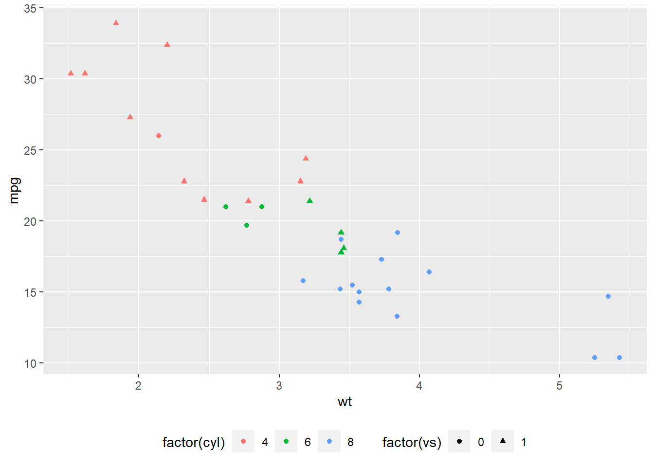

# Right -> inside the plot area
basic + theme(
    legend.position = c(.95, .95),
    legend.justification = c("right", "top"),
    legend.box.just = "right",
    legend.margin = margin(6, 6, 6, 6)
    )

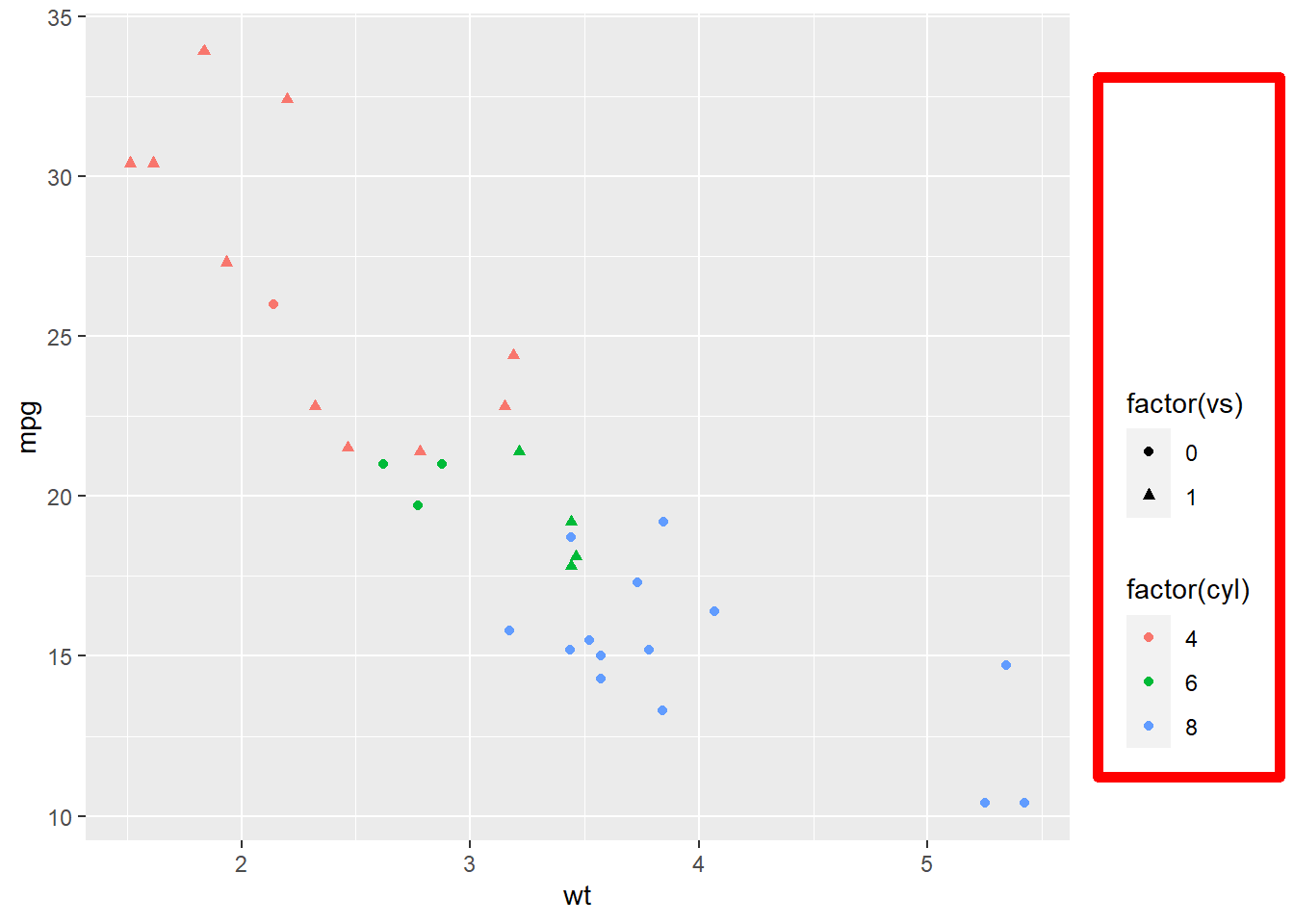
9.1.25 Legend Appearance

Here are 4 examples showing how to customize the legend main features:

• Box with legend.box.: it is a rectangle that frames the legend. Give features with element_rect().
• Key with legend.key: the key is the part showing the symbols. Note that symbols will automatically be the ones used on the chart.
• Text with legend.text: here you can control the color, the size of the right part of the legend.
• Title with legend.title.

# custom box around legend
basic + theme(
    legend.box.background = element_rect(color="red", size=2),
    legend.box.margin = margin(116, 6, 6, 6)
)

# custom the key
basic + theme(legend.key = element_rect(fill = "white", colour = "black"))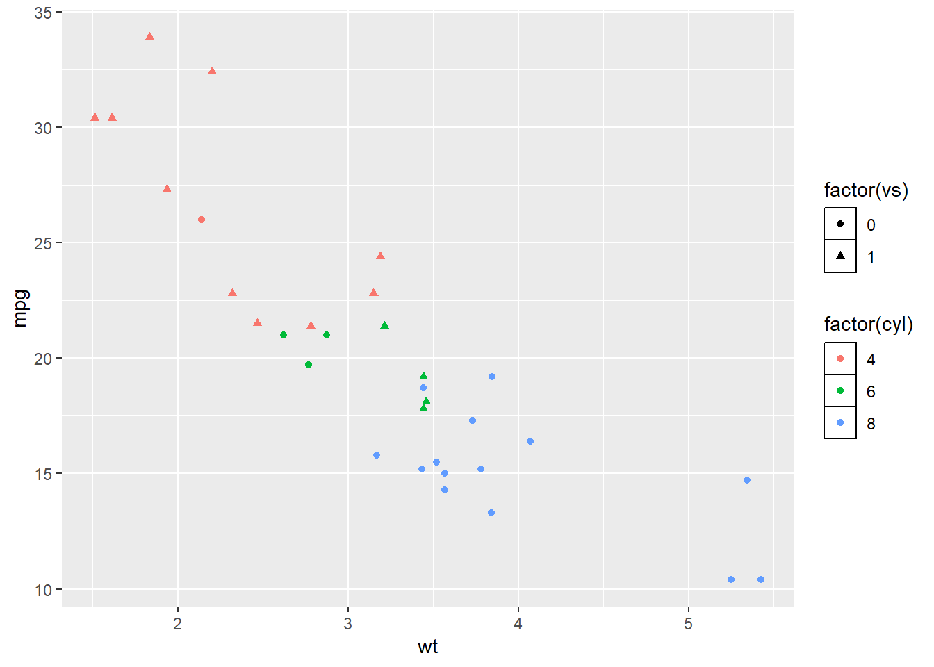

# custom the text
basic + theme(legend.text = element_text(size = 8, colour = "red"))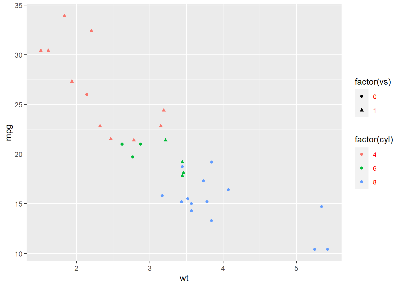

# custom the title
basic + theme(legend.title = element_text(face = "bold"))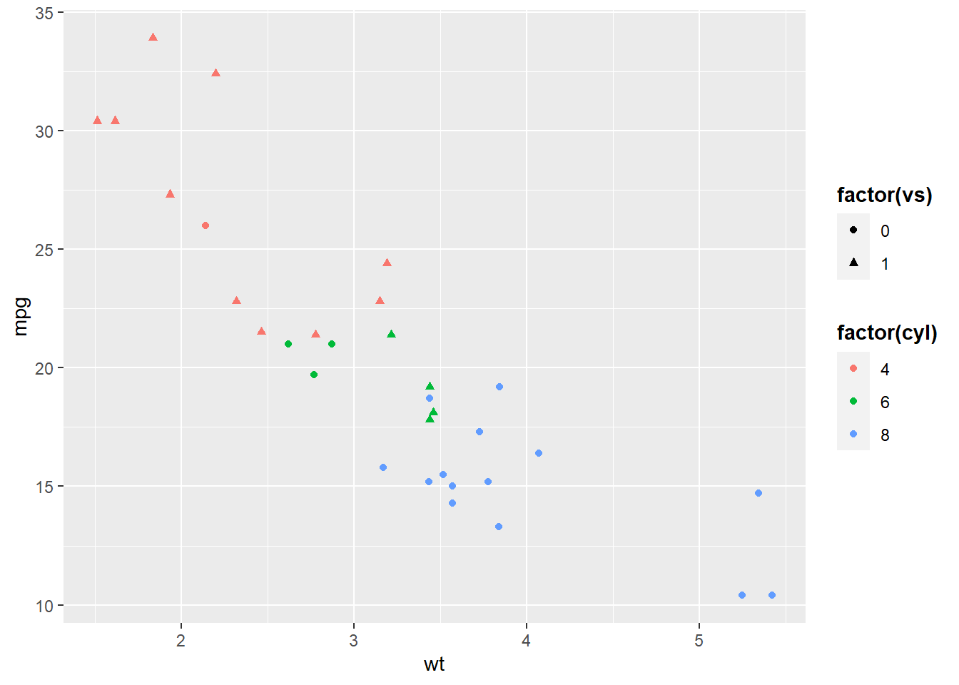

9.1.26 Reorder a Variable with ggplot2

This section describes how to reorder a variable in a ggplot2 chart. Several methods are suggested, always providing examples with reproducible code chunks.

Reordering groups in a ggplot2 chart can be a struggle. This is due to the fact that ggplot2 takes into account the order of the factor levels, not the order you observe in your data frame. You can sort your input data frame with sort() or arrange(), it will never have any impact on your ggplot2 output.

This post explains how to reorder the level of your factor through several examples. Examples are based on 2 dummy datasets:

# Library
library(ggplot2)
library(dplyr)

# Dataset 1: one value per group
data <- data.frame(
  name=c("north","south","south-east","north-west","south-west","north-east","west","east"),
  val=sample(seq(1,10), 8 )
)
 
# Dataset 2: several values per group (natively provided in R)
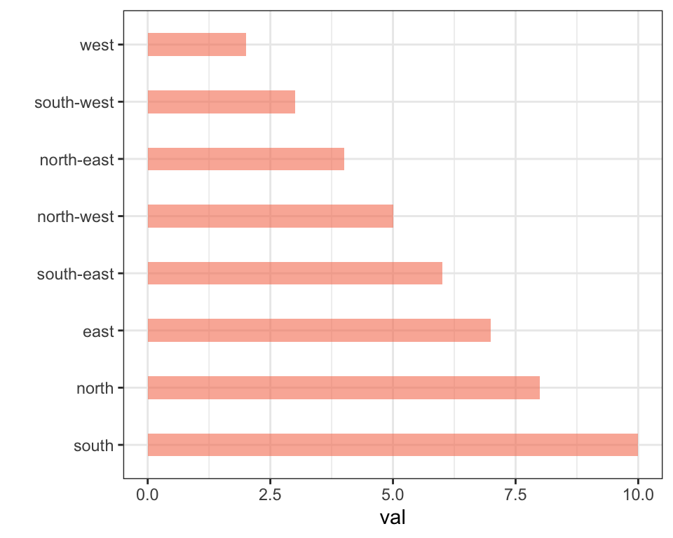
# mpg

9.1.27 Method 1: the Forecats library

The Forecats library is a library from the tidyverse especially made to handle factors in R. It provides a suite of useful tools that solve common problems with factors. The fact_reorder() function allows to reorder the factor (data$name for example) following the value of another column (data$val here).

# load the library
library(forcats)

# Reorder following the value of another column:
data %>%
  mutate(name = fct_reorder(name, val)) %>%
  ggplot( aes(x=name, y=val)) +
    geom_bar(stat="identity", fill="#f68060", alpha=.6, width=.4) +
    coord_flip() +
    xlab("") +
    theme_bw()
 
# Reverse side
data %>%
  mutate(name = fct_reorder(name, desc(val))) %>%
  ggplot( aes(x=name, y=val)) +
    geom_bar(stat="identity", fill="#f68060", alpha=.6, width=.4) +
    coord_flip() +
    xlab("") +
    theme_bw()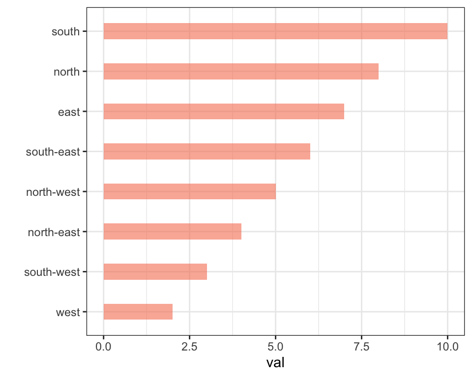

If you have several values per level of your factor, you can specify which function to apply to determine the order. The default is to use the median, but you can use the number of data points per group to make the classification:

# Using median
mpg %>%
  mutate(class = fct_reorder(class, hwy, .fun='median')) %>%
  ggplot( aes(x=reorder(class, hwy), y=hwy, fill=class)) + 
    geom_boxplot() +
    xlab("class") +
    theme(legend.position="none") +
    xlab("")
 
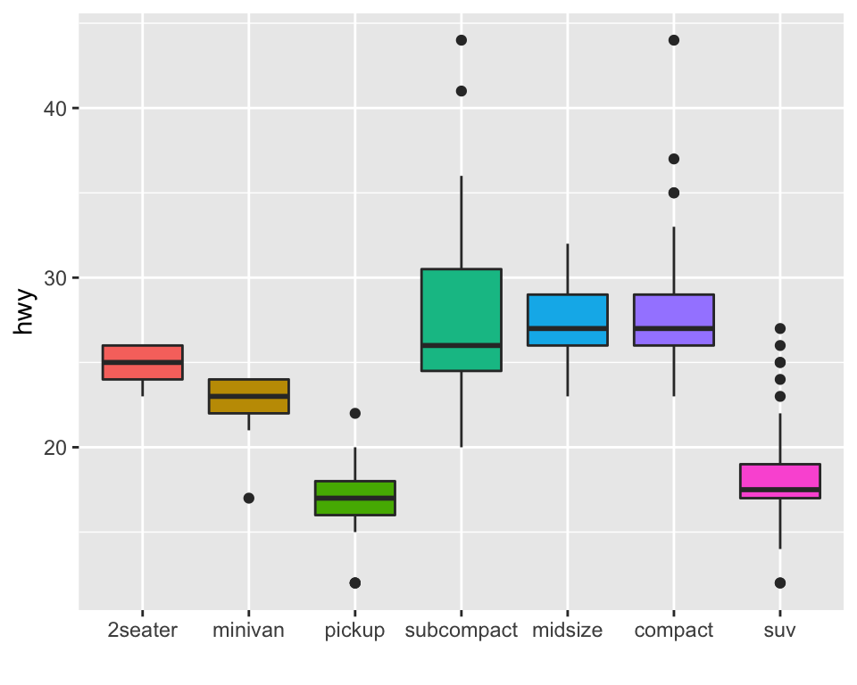
# Using number of observation per group
mpg %>%
  mutate(class = fct_reorder(class, hwy, .fun='length' )) %>%
  ggplot( aes(x=class, y=hwy, fill=class)) + 
    geom_boxplot() +
    xlab("class") +
    theme(legend.position="none") +
    xlab("") +
    xlab("")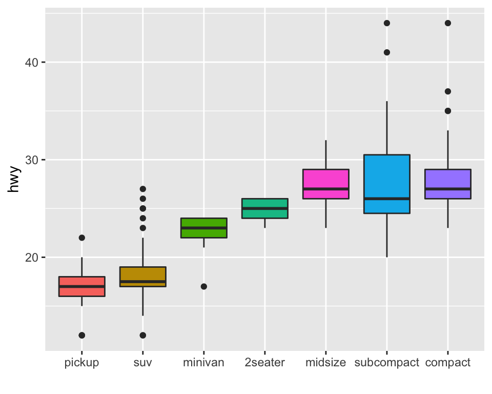

The last common operation is to provide a specific order to your levels, you can do so using the fct_relevel() function as follow:

# Reorder following a precise order
p <- data %>%
  mutate(name = fct_relevel(name, 
            "north", "north-east", "east", 
            "south-east", "south", "south-west", 
            "west", "north-west")) %>%
  ggplot( aes(x=name, y=val)) +
    geom_bar(stat="identity") +
    xlab("")
#p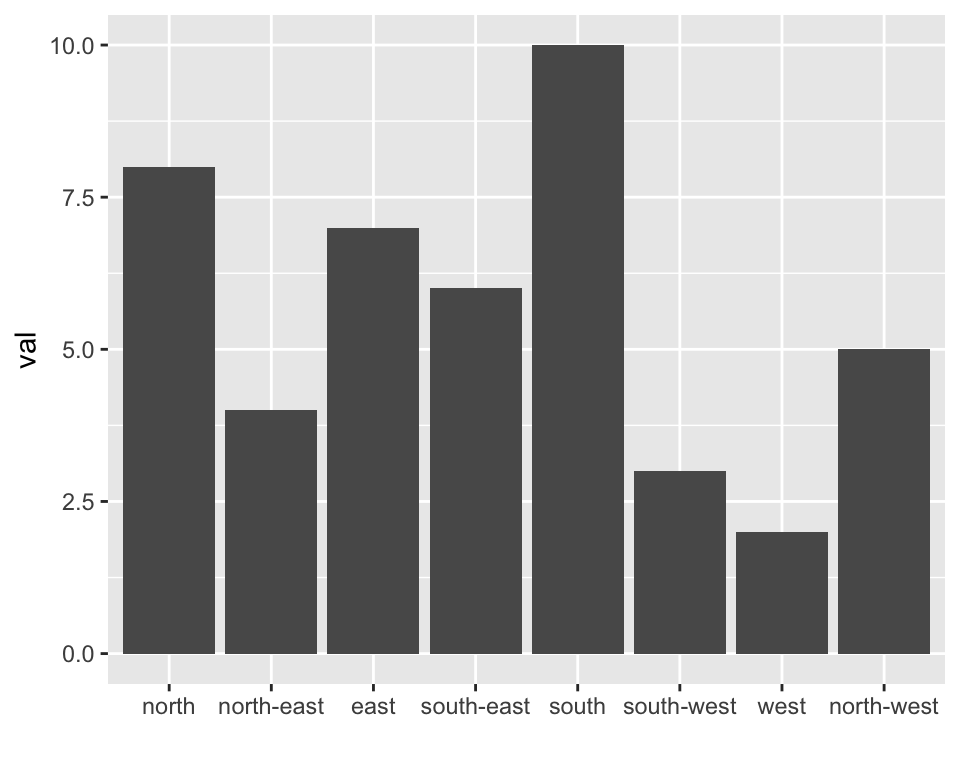

9.1.28 Method 2: Using dplyr Only

The mutate() function of dplyr allows to create a new variable or modify an existing one. It is possible to use it to recreate a factor with a specific order. Here are 2 examples:

• The first use arrange() to sort your data frame, and reorder the factor following this desired order.
• The second specifies a custom order for the factor giving the levels one by one.

data %>%
  arrange(val) %>%    # First sort by val. This sort the dataframe but NOT the factor levels
  mutate(name=factor(name, levels=name)) %>%   # This trick update the factor levels
  ggplot( aes(x=name, y=val)) +
    geom_segment( aes(xend=name, yend=0)) +
    geom_point( size=4, color="orange") +
    coord_flip() +
    theme_bw() +
    xlab("")
 
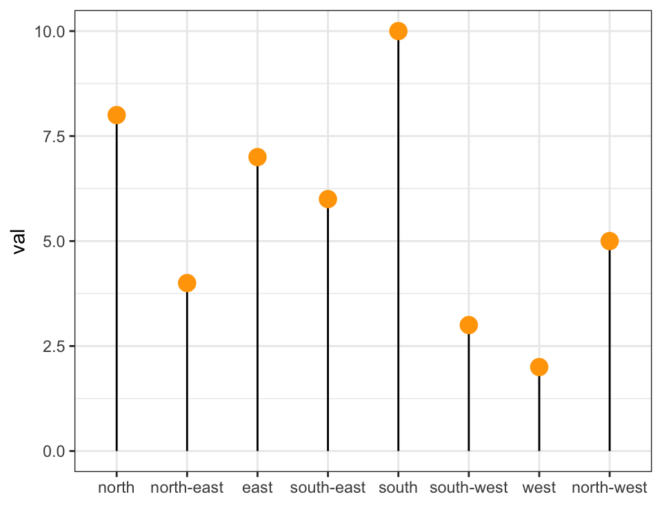
data %>%
  arrange(val) %>%
  mutate(name = factor(name, levels=c("north", "north-east", "east", "south-east", "south", "south-west", "west", "north-west"))) %>%
  ggplot( aes(x=name, y=val)) +
    geom_segment( aes(xend=name, yend=0)) +
    geom_point( size=4, color="orange") +
    theme_bw() +
    xlab("")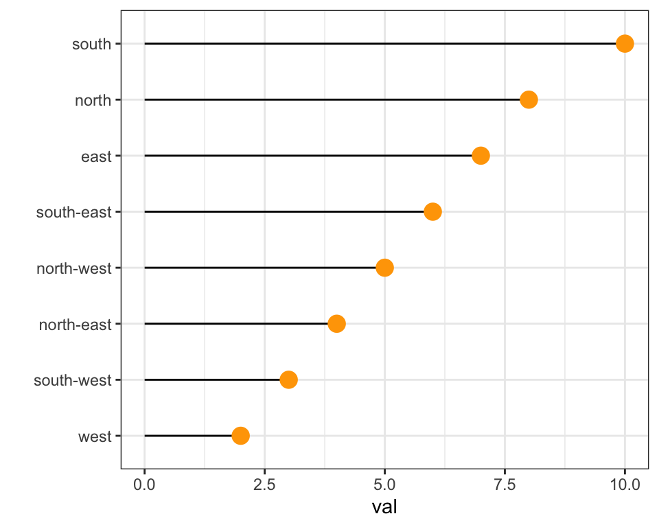

9.1.29 Method 3: the reorder() function of Base R

In case your an unconditional user of the good old R, here is how to control the order using the reorder() function inside a with() call:

# reorder is close to order, but is made to change the order of the factor levels.
mpg$class = with(mpg, reorder(class, hwy, median))

p <- mpg %>%
  ggplot( aes(x=class, y=hwy, fill=class)) + 
    geom_violin() +
    xlab("class") +
    theme(legend.position="none") +
    xlab("")
#p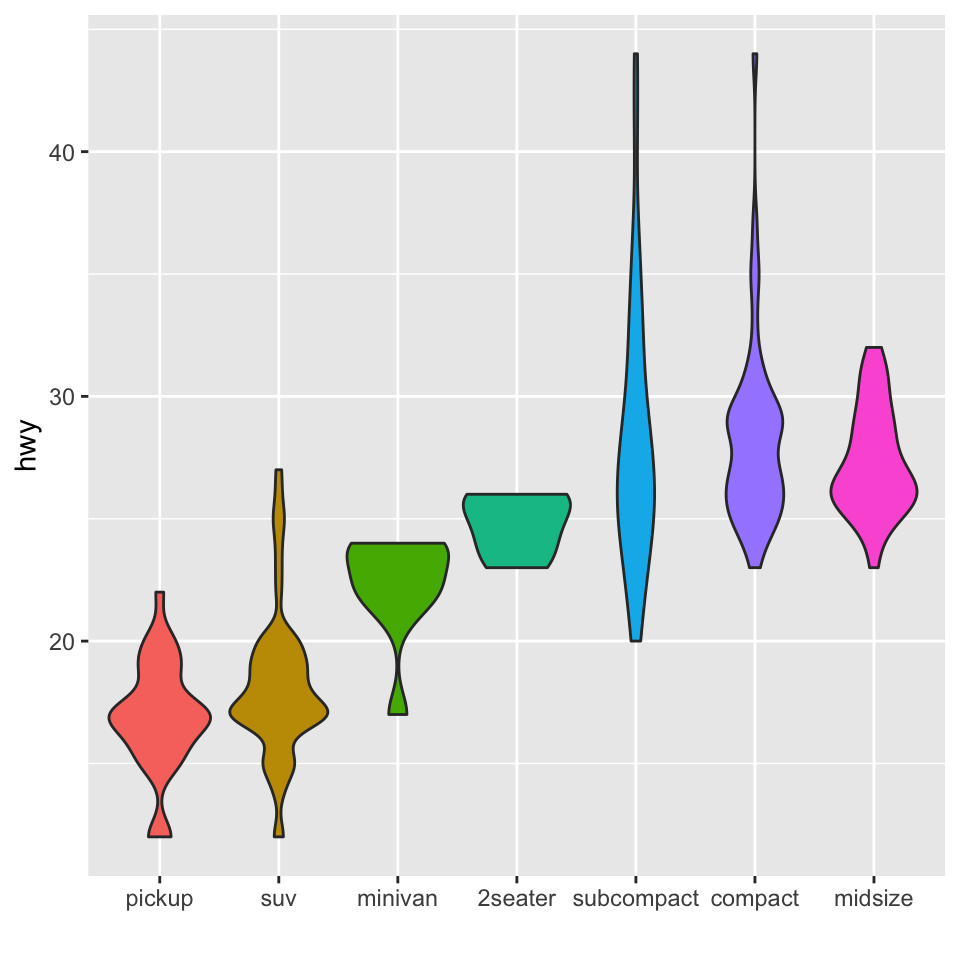

9.1.30 ggplot2 Title

The ggtitle() function allows to add a title to the chart. The following post will guide you through its usage, showing how to control title main features: position, font, color, text and more.

9.1.30.1 Title Manipulation with R and ggplot2

This section describes all the available options to customize the chart title with R and ggplot2. It shows how to control its color, its position, and more.

9.1.30.2 Default ggplot2 Title

It is possible to add a title to a ggplot2 chart using the ggtitle() function. It works as follow:

# library & data
library(ggplot2)
data <- data.frame(x=rnorm(100))
 
# Basic plot with title
ggplot( data=data, aes(x=x)) + 
  geom_histogram(fill="skyblue", alpha=0.5) +
  ggtitle("A blue Histogram") +
  theme_minimal()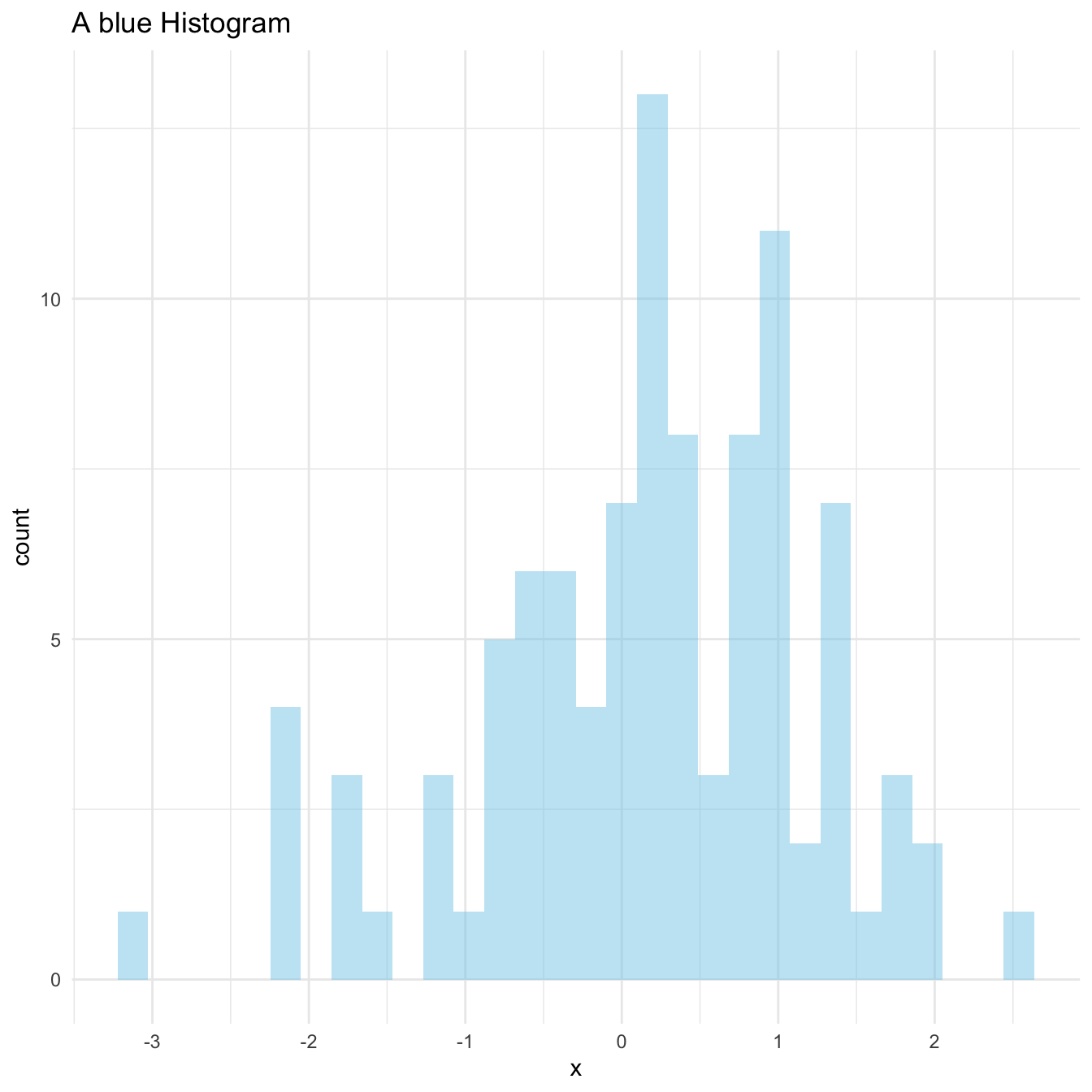

9.1.31 Title on Several Lines

It is a common need to set the title on several lines. To add a break and skip to a second line, just add a \n in the text.

# title on several lines
ggplot( data=data, aes(x=x)) + 
  geom_histogram(fill="skyblue", alpha=0.5) +
  ggtitle("A blue \nHistogram") +
  theme_minimal()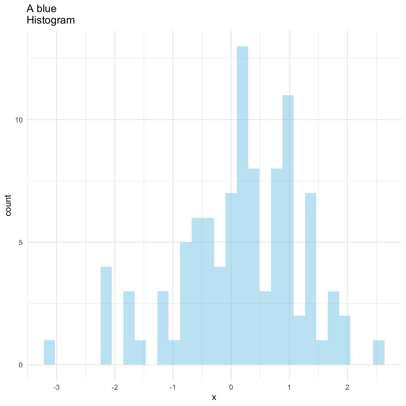 

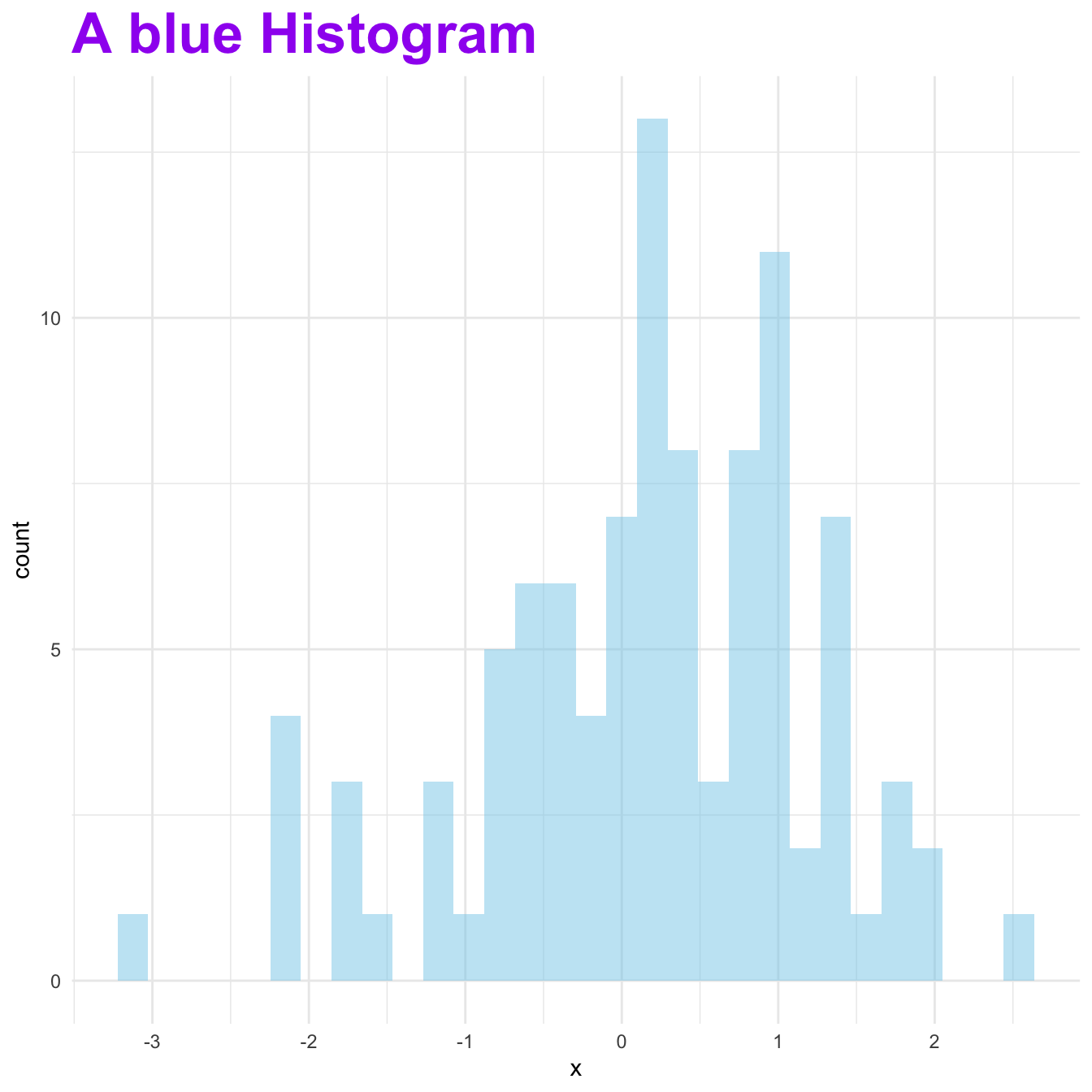
9.1.32 Title Appearance and Position

Here are 2 tricks to control text appearance and its position. Both features are controlled thanks to the plot.title argument of the theme() function. Appearance can be controlled with option such as family, size or color, when position is controlled with hjust and vjust.

# Custom title appearance
ggplot( data=data, aes(x=x)) + 
  geom_histogram(fill="skyblue", alpha=0.5) +
  ggtitle("A blue Histogram") +
  theme_minimal() +
  theme(
    plot.title=element_text(family='', face='bold', colour='purple', size=26)
  )

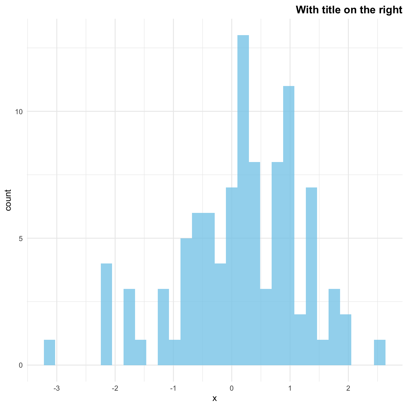
# Adjust the position of title
ggplot( data=data, aes(x=x)) + 
  geom_histogram(fill="skyblue", alpha=0.8) +
  ggtitle("With title on the right") +
  theme_minimal() +
  theme(
    plot.title=element_text( hjust=1, vjust=0.5, face='bold')
  )

9.1.33 Customize a Specific Word Only

If you want to highlight a specific set of words in the title, it is double thanks to the expression() function.

# Custom a few word of the title only:
my_title <- expression(paste("A ", italic(bold("blue")), " histogram"))
ggplot( data=data, aes(x=x)) + 
  geom_histogram(fill="skyblue", alpha=0.8) +
  ggtitle(my_title) +
  theme_minimal()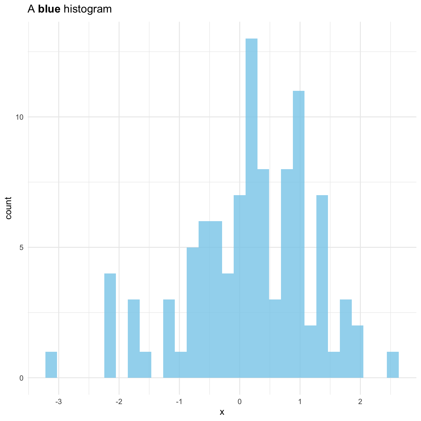

9.1.34 Small Multiples: facet_wrap() and facet_grid()

Small multiples is a very powerful dataviz technique. It split the chart window in many small similar charts: each represents a specific group of a categorical variable. The following post describes the main use cases using facet_wrap() and facet_grid() and should get you started quickly.

9.1.35 Faceting with ggplot2

This section describes all the available options to use small multiples with R and ggplot2. it shows how to efficiently split the chart window by row, column or both to show every group of the dataset separately.

9.1.35.1 What is Small Multiple

Faceting is the process that split the chart window in several small parts (a grid), and display a similar chart in each section. Each section usually shows the same graph for a specific group of the dataset. The result is usually called small multiple.

It is a very powerful technique in data visualization, and a major advantage of using ggplot2 is that it offers functions allowing to build it in a single line of code. Here is an example showing the evolution of a few baby names in the US. (source)

# Libraries
library(tidyverse)
library(hrbrthemes)
library(babynames)
library(viridis)

# Load dataset from github
data <- read.table("https://raw.githubusercontent.com/holtzy/data_to_viz/master/Example_dataset/3_TwoNumOrdered.csv", header=T)
data$date <- as.Date(data$date)

# Load dataset from github
don <- babynames %>% 
  filter(name %in% c("Ashley", "Amanda", "Mary", "Deborah",   "Dorothy", "Betty", "Helen", "Jennifer", "Shirley")) %>%
  filter(sex=="F")

# Plot
don %>%
  ggplot( aes(x=year, y=n, group=name, fill=name)) +
    geom_area() +
    scale_fill_viridis(discrete = TRUE) +
    theme(legend.position="none") +
    ggtitle("Popularity of American names in the previous 30 years") +
    theme_ipsum() +
    theme(
      legend.position="none",
      panel.spacing = unit(0, "lines"),
      strip.text.x = element_text(size = 8),
      plot.title = element_text(size=13)
    ) +
    facet_wrap(~name, scale="free_y")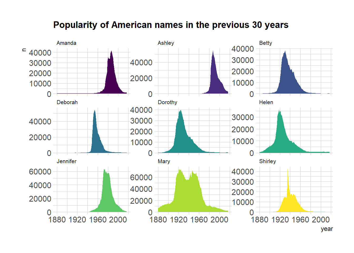

9.1.36 Faceting with facet_wrap()

facet_wrap() is the most common function for faceting with ggplot2. It builds a new chart for each level of a categorical variable. You can add the charts horizontally (graph1) or vertically (graph2, using dir="v"). Note that if the number of group is big enough, ggplot2 will automatically display charts on several rows/columns.

The grey bar showing the related level can be placed on top or on the bottom thanks to the strip.position option (graph3).

Last but not least, you can choose whether every graph have the same scale or not with the scales option (graph4).

# library & datset
library(ggplot2)
head(mtcars)

##                    mpg cyl disp  hp drat    wt  qsec vs am gear carb
## Mazda RX4         21.0   6  160 110 3.90 2.620 16.46  0  1    4    4
## Mazda RX4 Wag     21.0   6  160 110 3.90 2.875 17.02  0  1    4    4
## Datsun 710        22.8   4  108  93 3.85 2.320 18.61  1  1    4    1
## Hornet 4 Drive    21.4   6  258 110 3.08 3.215 19.44  1  0    3    1
## Hornet Sportabout 18.7   8  360 175 3.15 3.440 17.02  0  0    3    2
## Valiant           18.1   6  225 105 2.76 3.460 20.22  1  0    3    1

# Split by columns (default)
ggplot( mtcars , aes(x=mpg, y=wt, color=as.factor(cyl) )) + 
  geom_point(size=3) +  
  facet_wrap(~cyl) +
  theme(legend.position="none")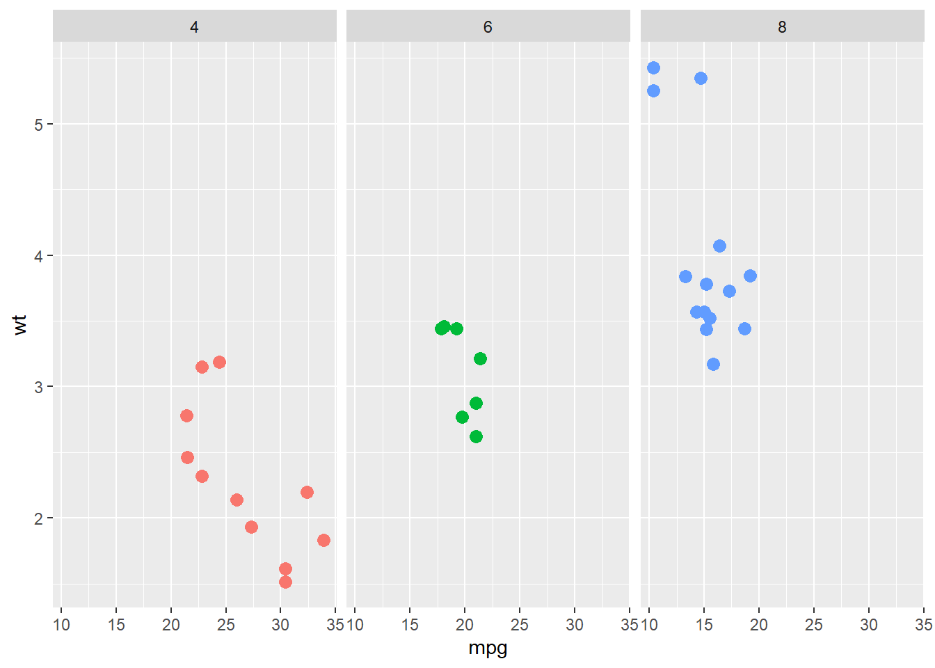

# Split by row
ggplot( mtcars , aes(x=mpg, y=wt, color=as.factor(cyl)  )) + 
  geom_point(size=3) +  
  facet_wrap(~cyl , dir="v")  +
  theme(legend.position="none")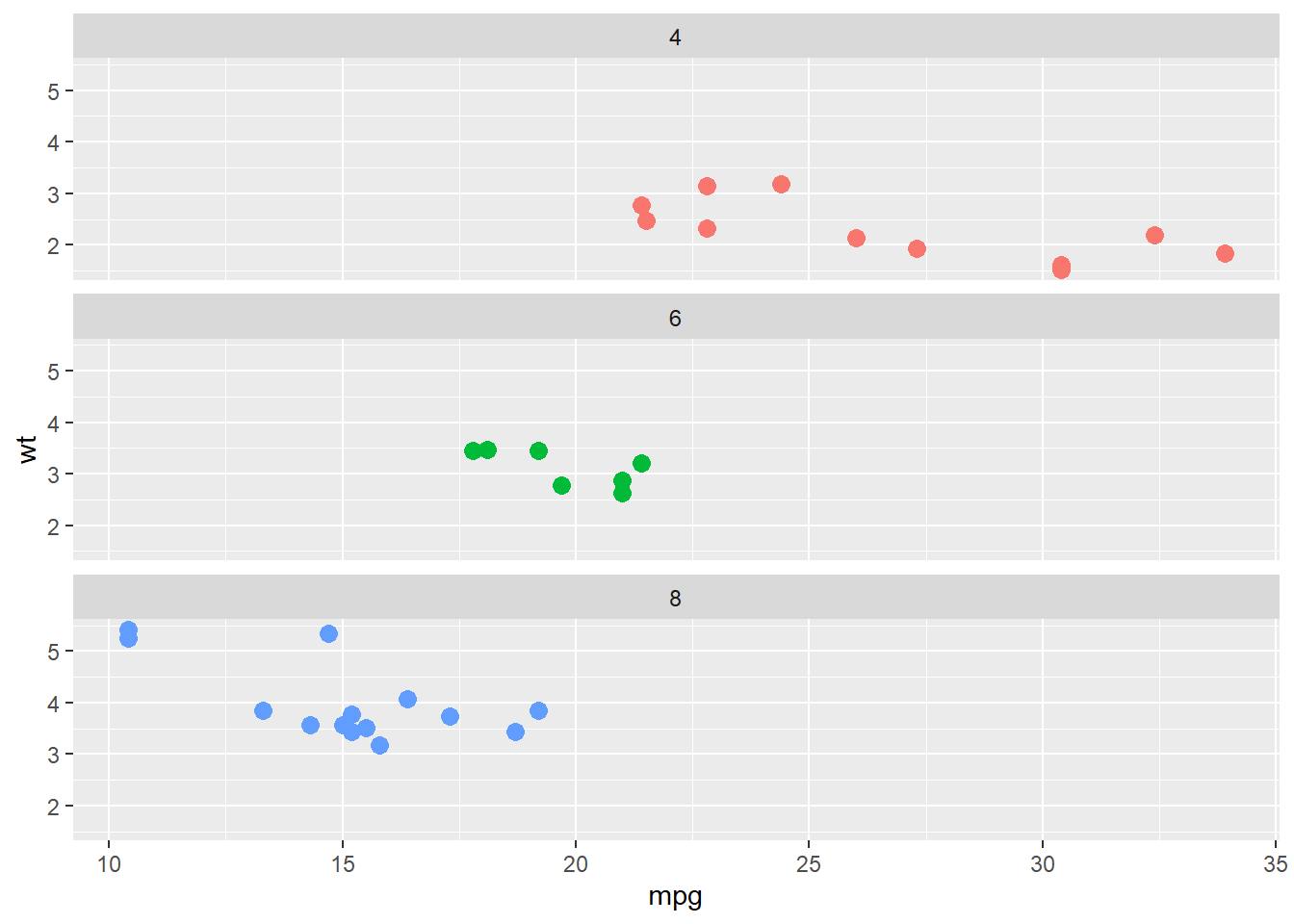

# Add label at the bottom
ggplot( mtcars , aes(x=mpg, y=wt, color=as.factor(cyl)  )) + 
  geom_point(size=3) +  
  facet_wrap(~cyl , strip.position="bottom") +
  theme(legend.position="none")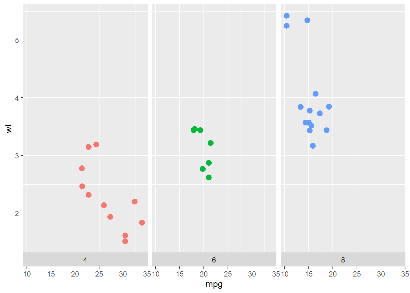

# Use same scales for all
ggplot( mtcars , aes(x=mpg, y=wt, color=as.factor(cyl)  )) + 
  geom_point(size=3) +  
  facet_wrap(~cyl , scales="free" ) +
  theme(legend.position="none")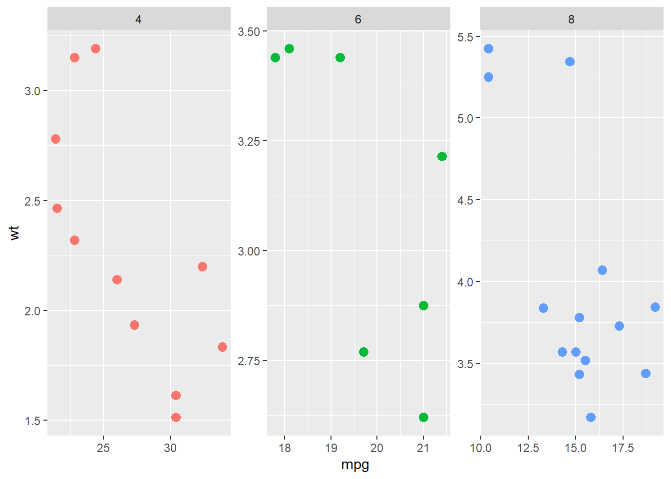

9.1.37 facet_grid()

facet_grid() is the second function allowing to build small multiples with ggplot2. It allows to build one chart for each combinations of 2 categorical variables. One variable will be used for rows, the other for columns.

The two variables must be given around a ~, the first being displayed as row, the second as column. The facet-grid() function also accepts the scales argument described above.

# Faceted ggplot2 using facet_grid():
ggplot( mtcars , aes(x=mpg, y=wt )) + 
  geom_point() +
  facet_grid( cyl ~ gear)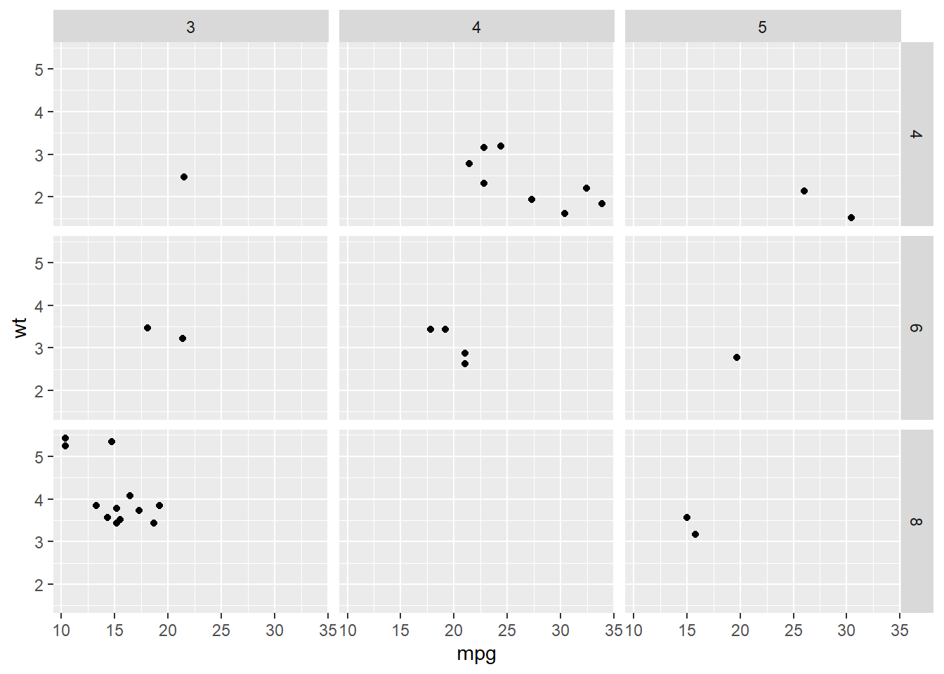

9.1.38 Customize Small Multiple Appearance with ggplot2

ggplot2 makes it a breeze to build small multiples. This post shows how to customize the layout, notably using the strip options

This section aims to provide useful R code to customize the strips of a ggplot2 plots when using faceting. For other ggplot2 customization, visit the dedicated page.

Here we want to modify non-data components, which is often done trough the theme() command. This page is strongly inspired from the help page of ggplot2 (?theme). Also, do not hesitate to visit the very strong ggplot2 documentation for more information.

Chart 1 is a really basic plot relying on the mtcars dataset. The 3 following charts show how to customize strip background, text, and how to modify the space between sections.

library(ggplot2)
 
# basic chart
basic=ggplot(mtcars, aes(wt, mpg)) +
    geom_point() +
    facet_wrap(~ cyl)
basic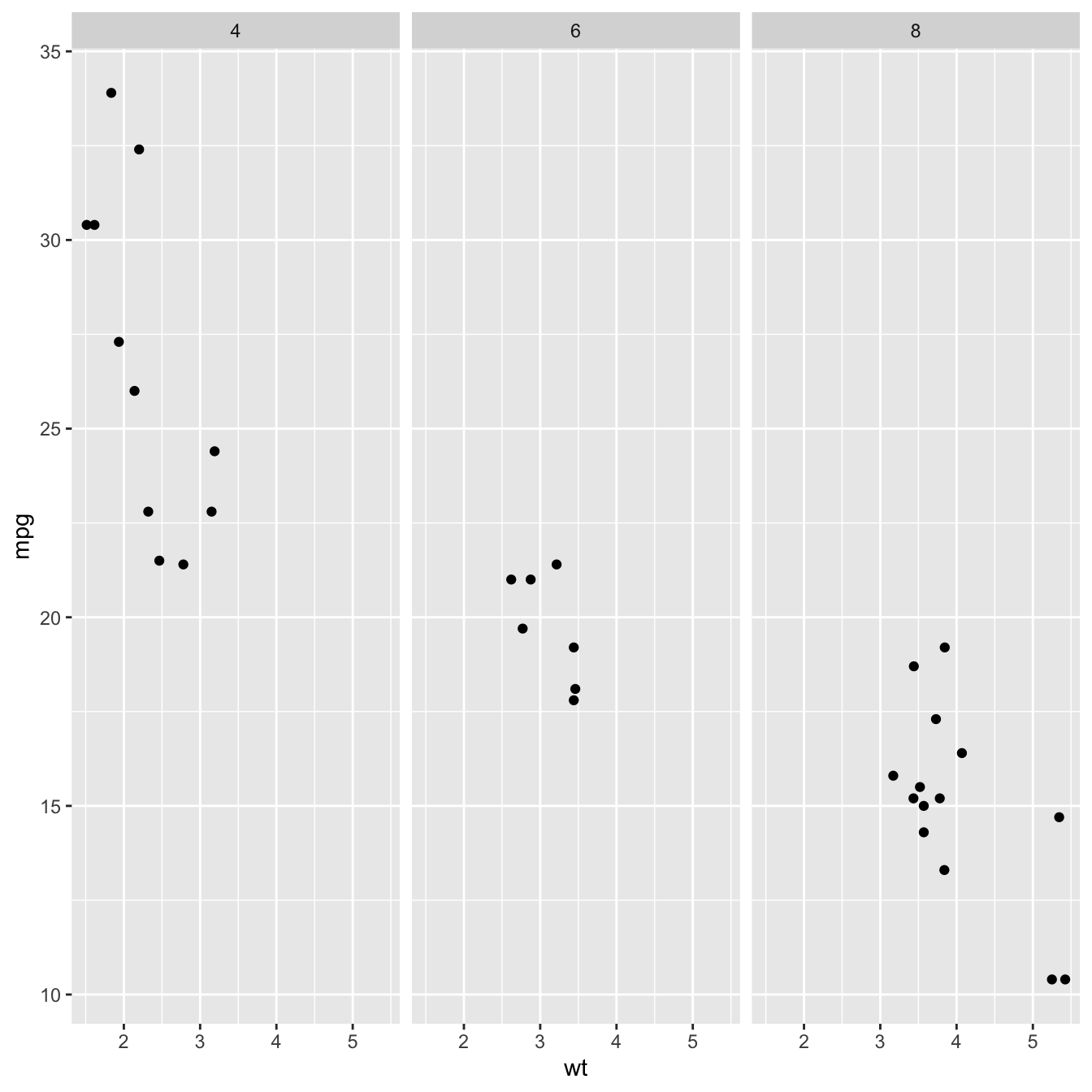

# Change background
basic + theme(strip.background = element_rect(colour = "red", fill = alpha("blue",0.2) ))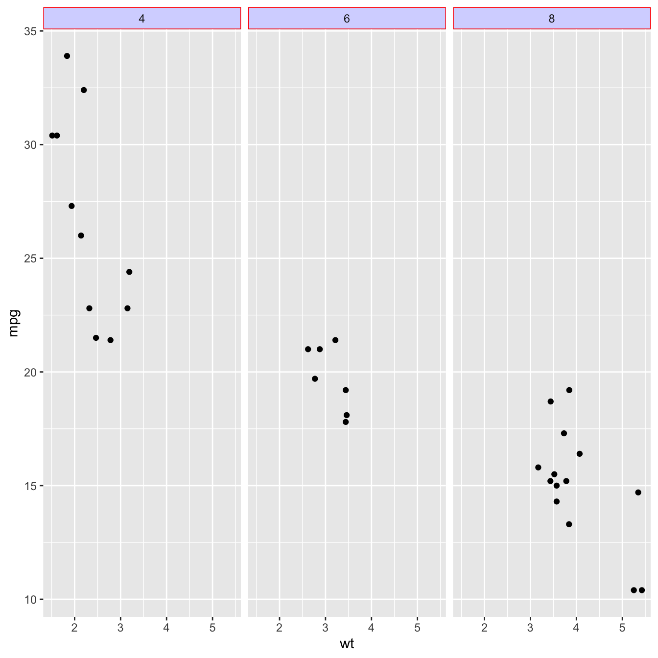

# Change the text 
basic + theme(strip.text.x = element_text(colour = "red", face = "bold", size=10, angle=30))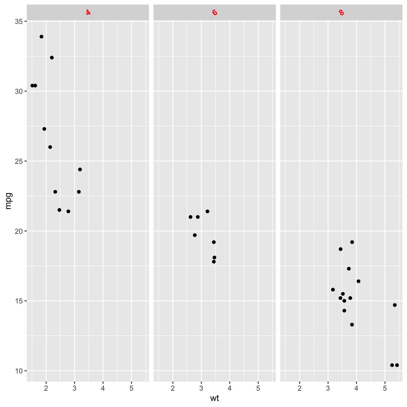

# Change the space between parts:
basic + theme(panel.spacing = unit(4, "lines"))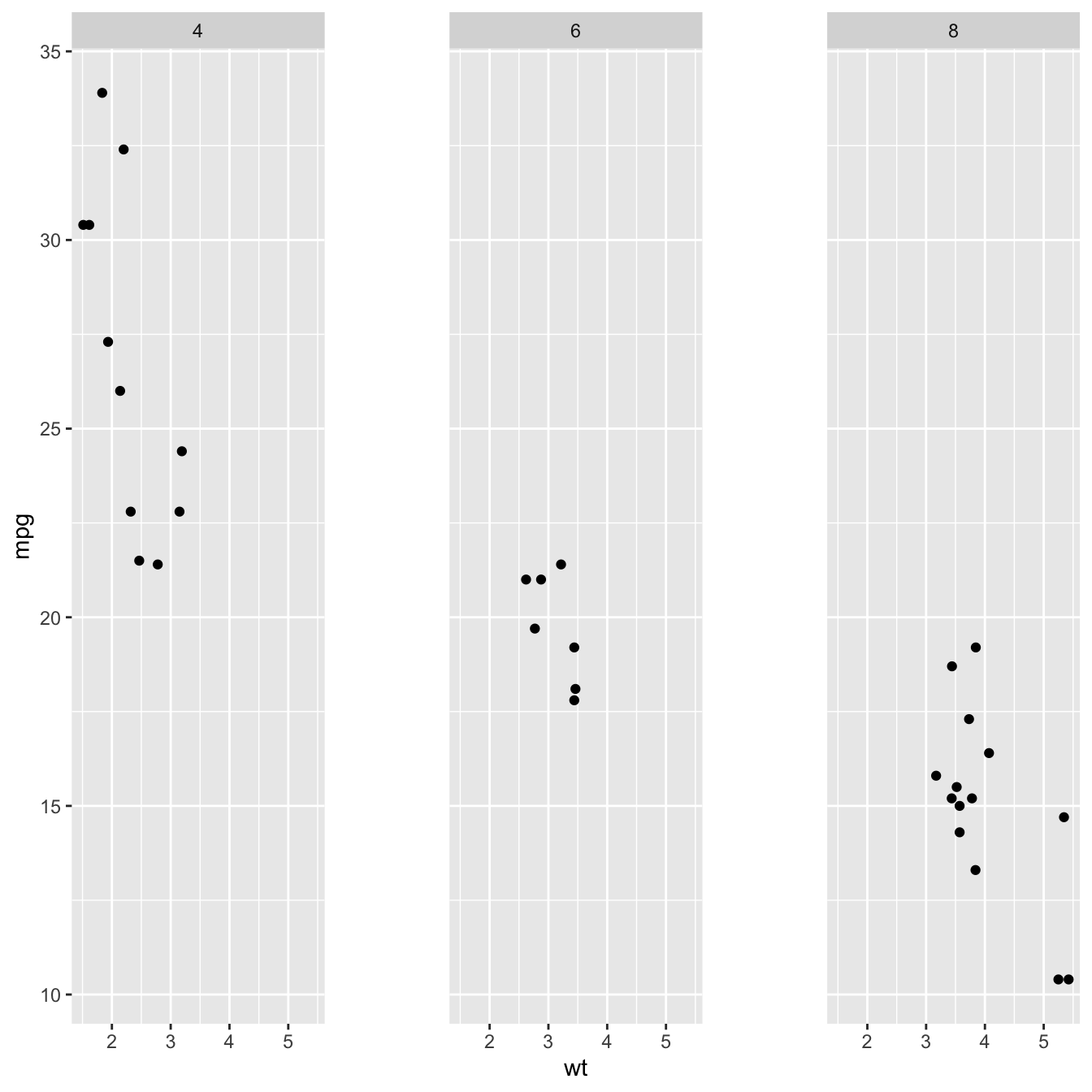

9.1.39 Multiple ggplot2 Charts on a Single Page

This section shows how to use the gridExtra library to combine several ggplot2 charts on the same figure. Several examples are provided, illustrating several ways to split the graphing window.

Mixing multiple graphs on the same page is a common practice. It allows to summarize a lot of information on the same figure, and is for instance widely used for scientific publication.

The gridExtra package makes it a breeze. It offers the grid.arrange() function that does exactly that. Its nrow argument allows to specify how to arrange the layout.

For more complex layout, the arrangeGrob() functions allows to do some nesting. Here are 4 examples to illustrate how gridExtra works:

# libraries
library(ggplot2)
library(gridExtra)
 
# Make 3 simple graphics:
g1 <- ggplot(mtcars, aes(x=qsec)) + geom_density(fill="slateblue")
g2 <- ggplot(mtcars, aes(x=drat, y=qsec, color=cyl)) + geom_point(size=5) + theme(legend.position="none")
g3 <- ggplot(mtcars, aes(x=factor(cyl), y=qsec, fill=cyl)) + geom_boxplot() + theme(legend.position="none")
g4 <- ggplot(mtcars , aes(x=factor(cyl), fill=factor(cyl))) +  geom_bar()
 
# Plots
grid.arrange(g2, arrangeGrob(g3, g4, ncol=2), nrow = 2)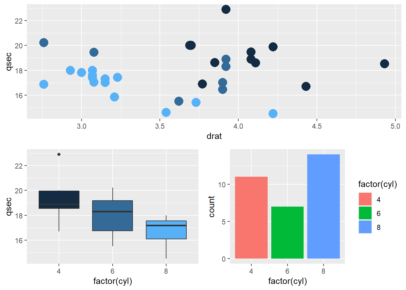

grid.arrange(g1, g2, g3, nrow = 3)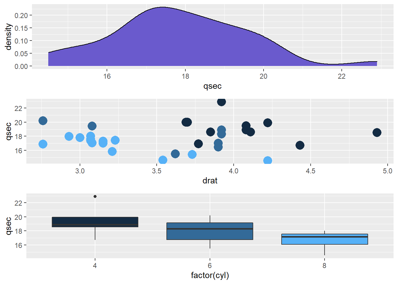

grid.arrange(g2, arrangeGrob(g3, g4, ncol=2), nrow = 1)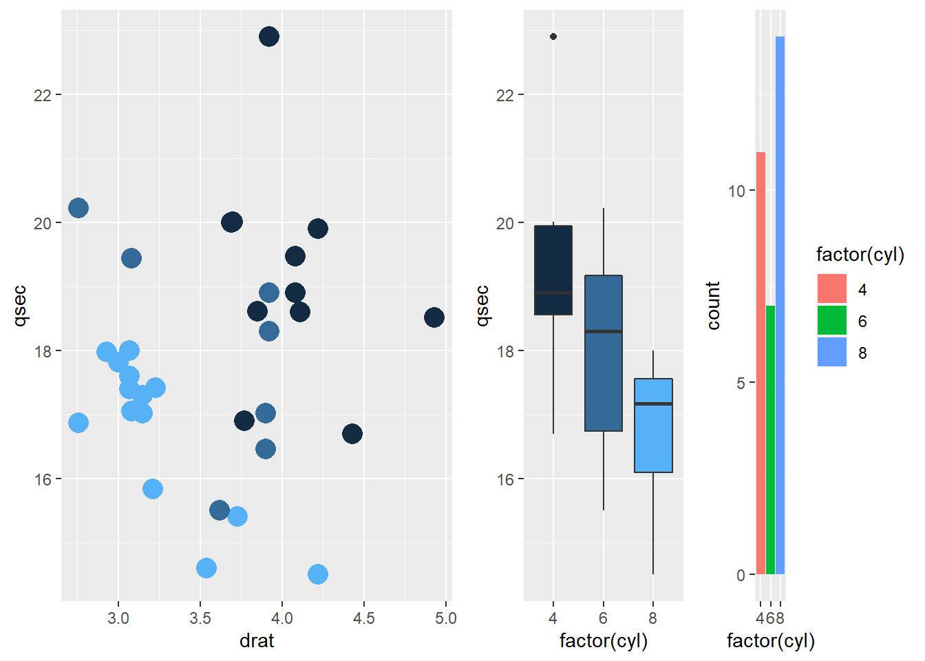

grid.arrange(g2, arrangeGrob(g3, g4, nrow=2), nrow = 1)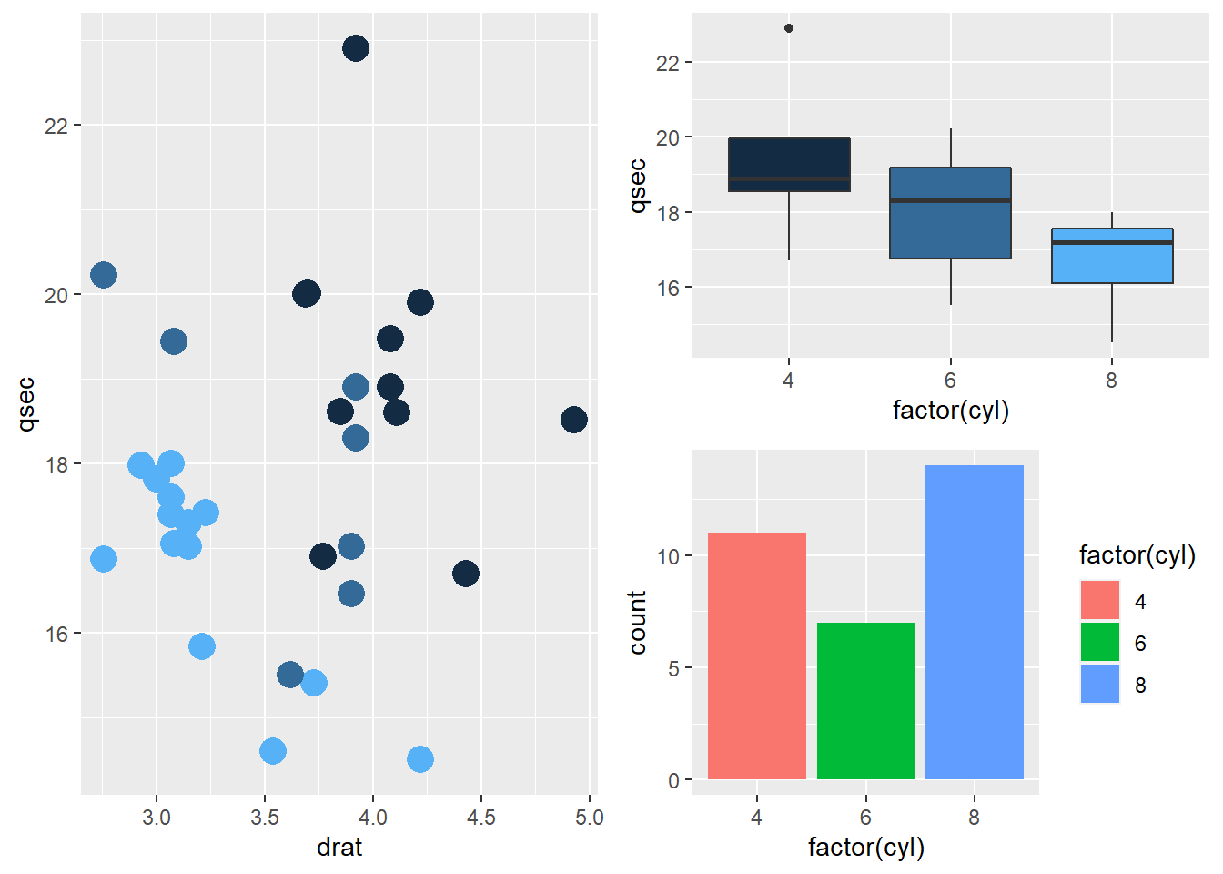

9.1.40 Plotly: Turn your ggplot Interactive

Another awesome feature of ggplot2 is its link with the plotly library. If you know how to make a ggplot2 chart, you are 10 seconds away to rendering an interactive version. Just call the ggplotly() function, and you’re done. Visit the interactive graphic section of the gallery for more.

library(ggplot2)
library(plotly)
library(gapminder)

p <- gapminder %>%
  filter(year==1977) %>%
  ggplot( aes(gdpPercap, lifeExp, size = pop, color=continent)) +
  geom_point() +
  theme_bw()

ggplotly(p)

AN OVERVIEW OF GGPLOT2 POSSIBILITIES

9.1.41 An Overview of ggplot2 Possibilities

Each section of the gallery provides several examples implemented with ggplot2. Here is an overview of my favorite examples:

9.1.41.1 Violin Plot with included Boxplot and Sample Size in ggplot2

It can be handy to include a boxplot in the violin plot to see both the distribution of the data and its summary statistics. Moreover, adding sample size of each group on the X axis is often a necessary step. Here is how to do it with R and ggplot2.

Building a violin plot with ggplot2 is pretty straightforward thanks to the dedicated geom_violin() function. It is possible to use geom_boxplot() with a small width in addition to display a boxplot that provides summary statistics.

Moreover, note a small trick that allows to provide sample size of each group on the X axis: a new column called myaxis is created and is then used for the X axis.

# Libraries
library(ggplot2)
library(dplyr)
library(hrbrthemes)
library(viridis)

# create a dataset
data <- data.frame(
  name=c( rep("A",500), rep("B",500), rep("B",500), rep("C",20), rep('D', 100)  ),
  value=c( rnorm(500, 10, 5), rnorm(500, 13, 1), rnorm(500, 18, 1), rnorm(20, 25, 4), rnorm(100, 12, 1) )
)

# sample size
sample_size = data %>% group_by(name) %>% summarize(num=n())

# Plot
data %>%
  left_join(sample_size) %>%
  mutate(myaxis = paste0(name, "\n", "n=", num)) %>%
  ggplot( aes(x=myaxis, y=value, fill=name)) +
    geom_violin(width=1.4) +
    geom_boxplot(width=0.1, color="grey", alpha=0.2) +
    scale_fill_viridis(discrete = TRUE) +
    theme_ipsum() +
    theme(
      legend.position="none",
      plot.title = element_text(size=11)
    ) +
    ggtitle("A Violin wrapping a boxplot") +
    xlab("")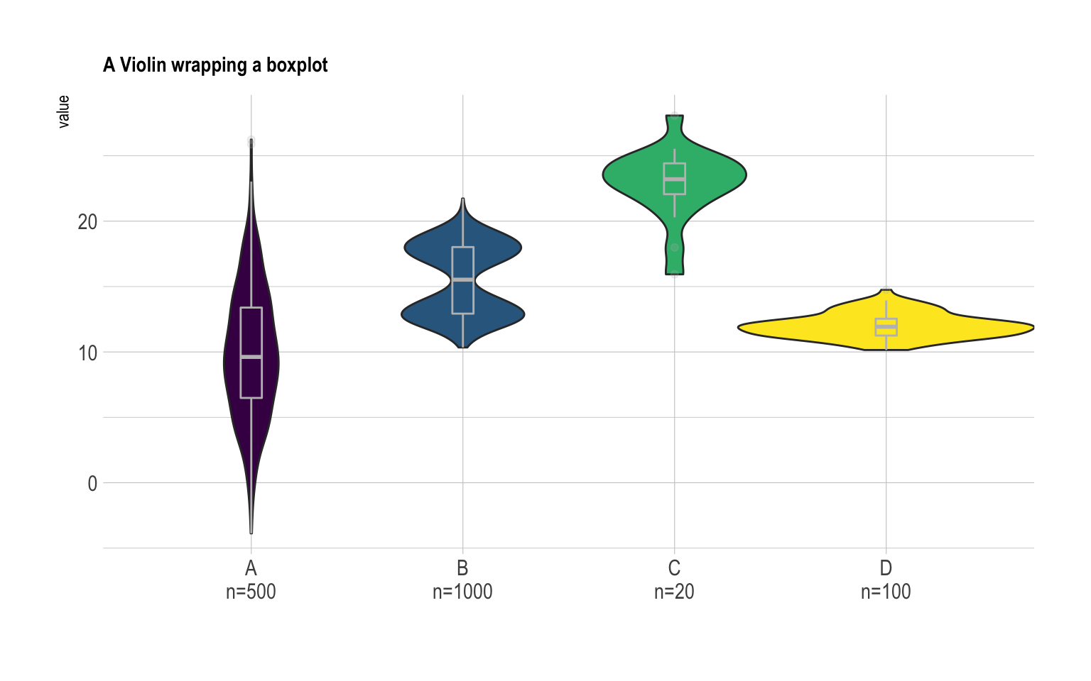

9.1.42 Boxplot with Individual Data Points

A boxplot summarizes the distribution of a continuous variable. it is often criticized for hiding the underlying distribution of each group. Thus, showing individual observation using jitter on top of boxes is a good practice. This post explains how to do so using ggplot2.

If you’re not convinced about that danger of using basic boxplot, please read this post that explains it in depth.

Fortunately, ggplot2 makes it a breeze to add invdividual observation on top of boxes thanks to the geom_jitter() function. This function shifts all dots by a random value ranging from 0 to size, avoiding overlaps.

Now, do you see the bimodal distribution hidden behind group B?

# Libraries
library(tidyverse)
library(hrbrthemes)
library(viridis)

# create a dataset
data <- data.frame(
  name=c( rep("A",500), rep("B",500), rep("B",500), rep("C",20), rep('D', 100)  ),
  value=c( rnorm(500, 10, 5), rnorm(500, 13, 1), rnorm(500, 18, 1), rnorm(20, 25, 4), rnorm(100, 12, 1) )
)

# Plot
data %>%
  ggplot( aes(x=name, y=value, fill=name)) +
    geom_boxplot() +
    scale_fill_viridis(discrete = TRUE, alpha=0.6) +
    geom_jitter(color="black", size=0.4, alpha=0.9) +
    theme_ipsum() +
    theme(
      legend.position="none",
      plot.title = element_text(size=11)
    ) +
    ggtitle("A boxplot with jitter") +
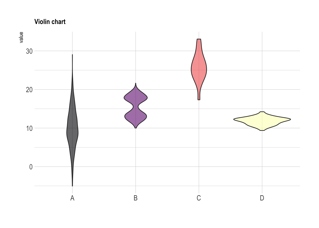
    xlab("")

In case you’re not convinced, here is how the basic boxplot and the basic violin plot look like:

# Boxplot basic
data %>%
  ggplot( aes(x=name, y=value, fill=name)) +
    geom_boxplot() +
    scale_fill_viridis(discrete = TRUE, alpha=0.6, option="A") +
    theme_ipsum() +
    theme(
      legend.position="none",
      plot.title = element_text(size=11)
    ) +
    ggtitle("Basic boxplot") +
    xlab("")

# Violin basic
data %>%
  ggplot( aes(x=name, y=value, fill=name)) +
    geom_violin() +
    scale_fill_viridis(discrete = TRUE, alpha=0.6, option="A") +
    theme_ipsum() +
    theme(
      legend.position="none",
      plot.title = element_text(size=11)
    ) +
    ggtitle("Violin chart") +
    xlab("")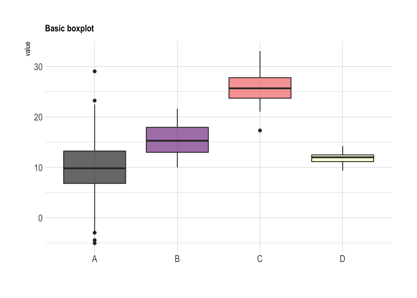

9.1.43 Map a Variable to Marker Feature in ggplot2 Scatterplot

ggplot2 allows to easily map a variable to marker features of a scatterplot. This post explaines how it works through several examples, with explanation and code.

9.1.44 Basic Example

Here is the magick of ggplot2: the ability to map a variable to marker features. Here, the marker color depends on its value in the field called Species in the input data frame.

Note that the legend is built automatically.

# load ggplot2
library(ggplot2)
library(hrbrthemes)

# mtcars dataset is natively available in R
# head(mtcars)
 
# A basic scatterplot with color depending on Species
ggplot(iris, aes(x=Sepal.Length, y=Sepal.Width, color=Species)) + 
    geom_point(size=6) +
    theme_ipsum()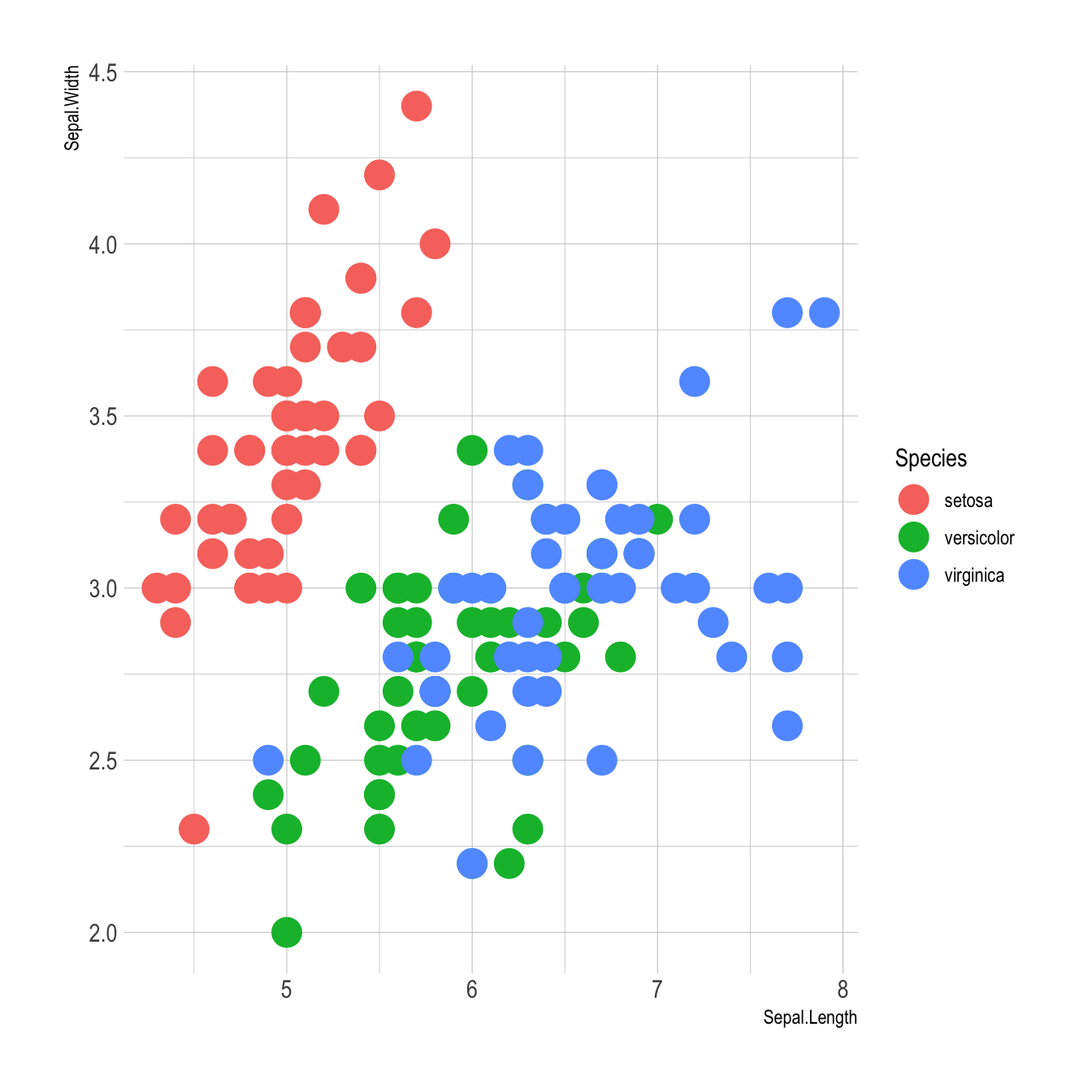

9.1.45 Works with any Aesthetics

You can map variables to any marker features. For instance, specie is represent below using transparency (left), shape (middle) and size (right).

# load ggplot2
library(ggplot2)
library(hrbrthemes)

# Transparency
ggplot(iris, aes(x=Sepal.Length, y=Sepal.Width, alpha=Species)) + 
    geom_point(size=6, color="#69b3a2") +
    theme_ipsum()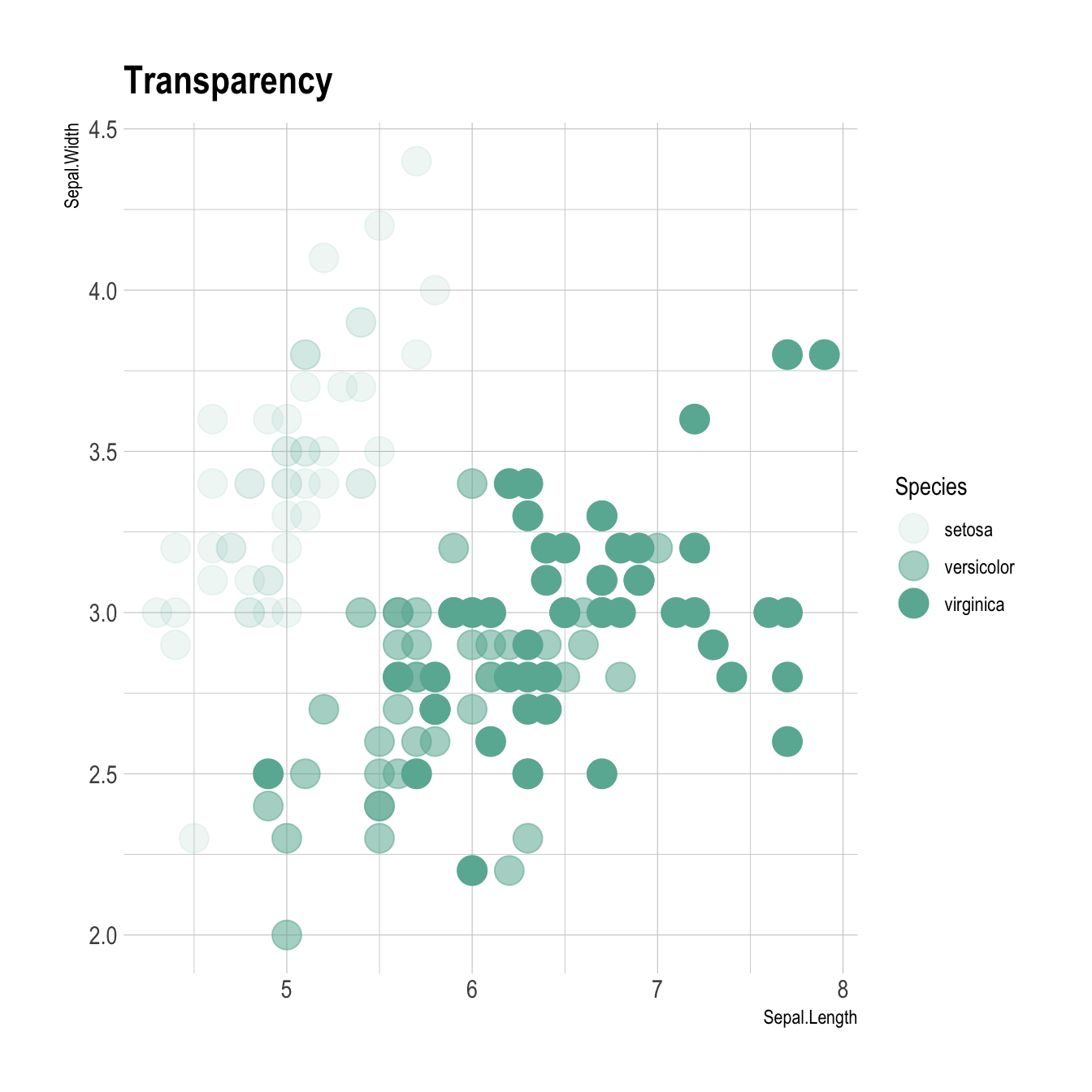

# Shape
ggplot(iris, aes(x=Sepal.Length, y=Sepal.Width, shape=Species)) + 
    geom_point(size=6) +
    theme_ipsum()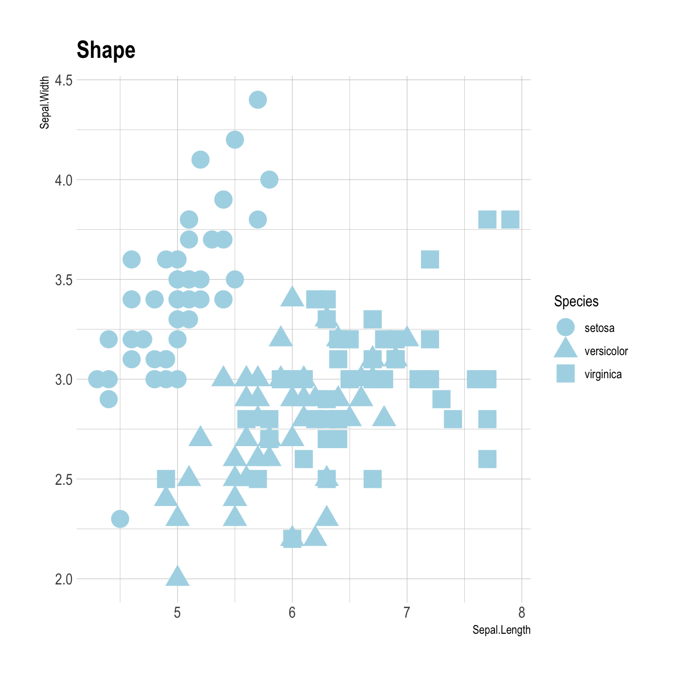

# Size
ggplot(iris, aes(x=Sepal.Length, y=Sepal.Width, shape=Species)) + 
    geom_point(size=6) +
    theme_ipsum()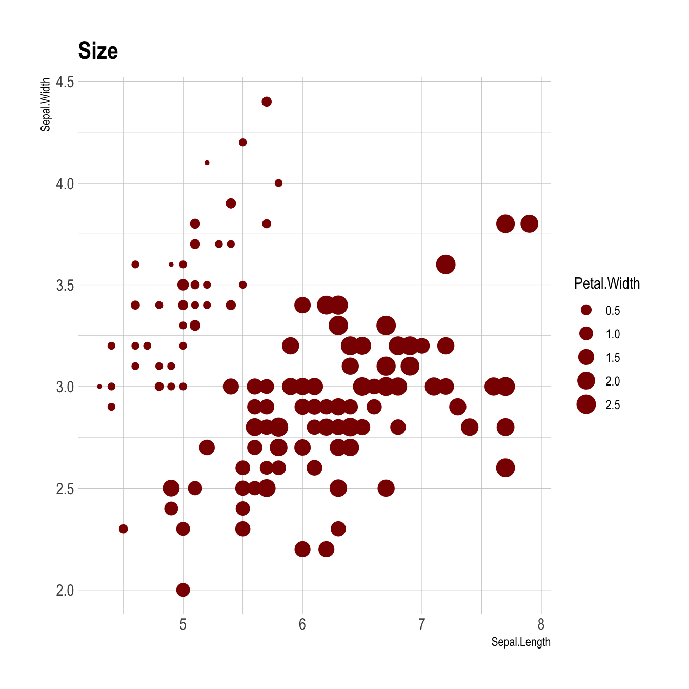

9.1.46 Mapping to Several Features

Last but not least, note that you can map one or several variables to one or several features. Here, shape, transparency, size and color all depends on the marker Species value.

# load ggplot2
library(ggplot2)
library(hrbrthemes)

# A basic scatterplot with color depending on Species
ggplot(iris, aes(x=Sepal.Length, y=Sepal.Width, shape=Species, alpha=Species, size=Species, color=Species)) + 
    geom_point() +
    theme_ipsum()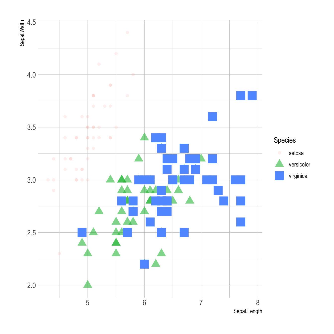

9.1.47 Bubble Plot with ggplot2

This section explains how to build a bubble chart with R and ggplot2. It provides several reproducible examples with explanation and R code.

9.1.47.1 Most Basic Bubble Chart with geom_point()

A bubble plot is a scatterplot where a third dimension is added: the value of an additional numeric variable is represented through the size of the dots. (source: data-to-viz).

With ggplot2, bubble chart are built thanks to the geom_point() function. At least three variable must be provided to aes(): x, y and size. The legend will automatically be built by ggplot2.

Here, the relationship between life expectancy (y) and gdp per capita (x) of world countries is represented. The population of each country is represented through circle size.

# Libraries
library(ggplot2)
library(dplyr)

# The dataset is provided in the gapminder library
library(gapminder)
data <- gapminder %>% filter(year=="2007") %>% dplyr::select(-year)

# Most basic bubble plot
ggplot(data, aes(x=gdpPercap, y=lifeExp, size = pop)) +
    geom_point(alpha=0.7)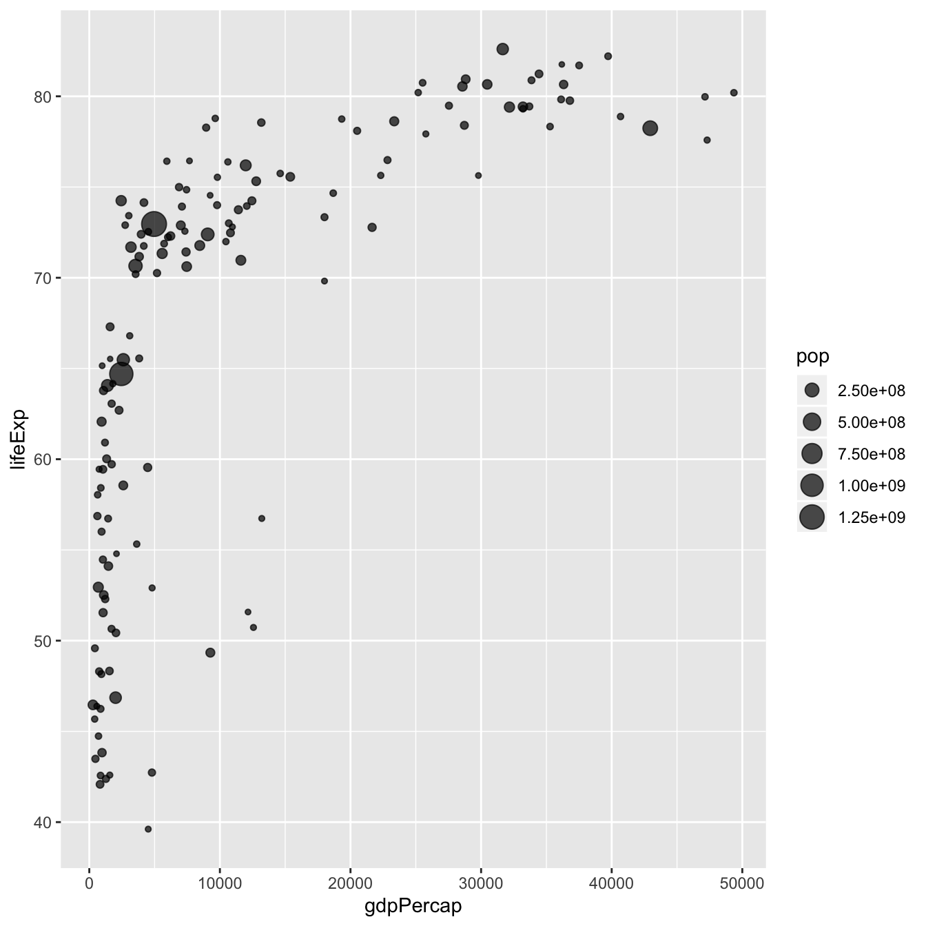

9.1.48 Control Circle Size with scale_size()

The first thing we need to improve on the previous chart is the bubble size. scale_size() allows to set the size of the smallest and the biggest circles using the range argument. Note that you can customize the legend name with name.

Note: Circles often overlap. To avoid having big circles on top of the chart you have to reorder your dataset first, as in the code below.

ToDo: Give more details about how to map a numeric variable to circle size. Use of scale_radius, scale_size and scale_size_area. See this post.

# Libraries
library(ggplot2)
library(dplyr)

# The dataset is provided in the gapminder library
library(gapminder)
data <- gapminder %>% filter(year=="2007") %>% dplyr::select(-year)

# Most basic bubble plot
data %>%
  arrange(desc(pop)) %>%
  mutate(country = factor(country, country)) %>%
  ggplot(aes(x=gdpPercap, y=lifeExp, size = pop)) +
    geom_point(alpha=0.5) +
    scale_size(range = c(.1, 24), name="Population (M)")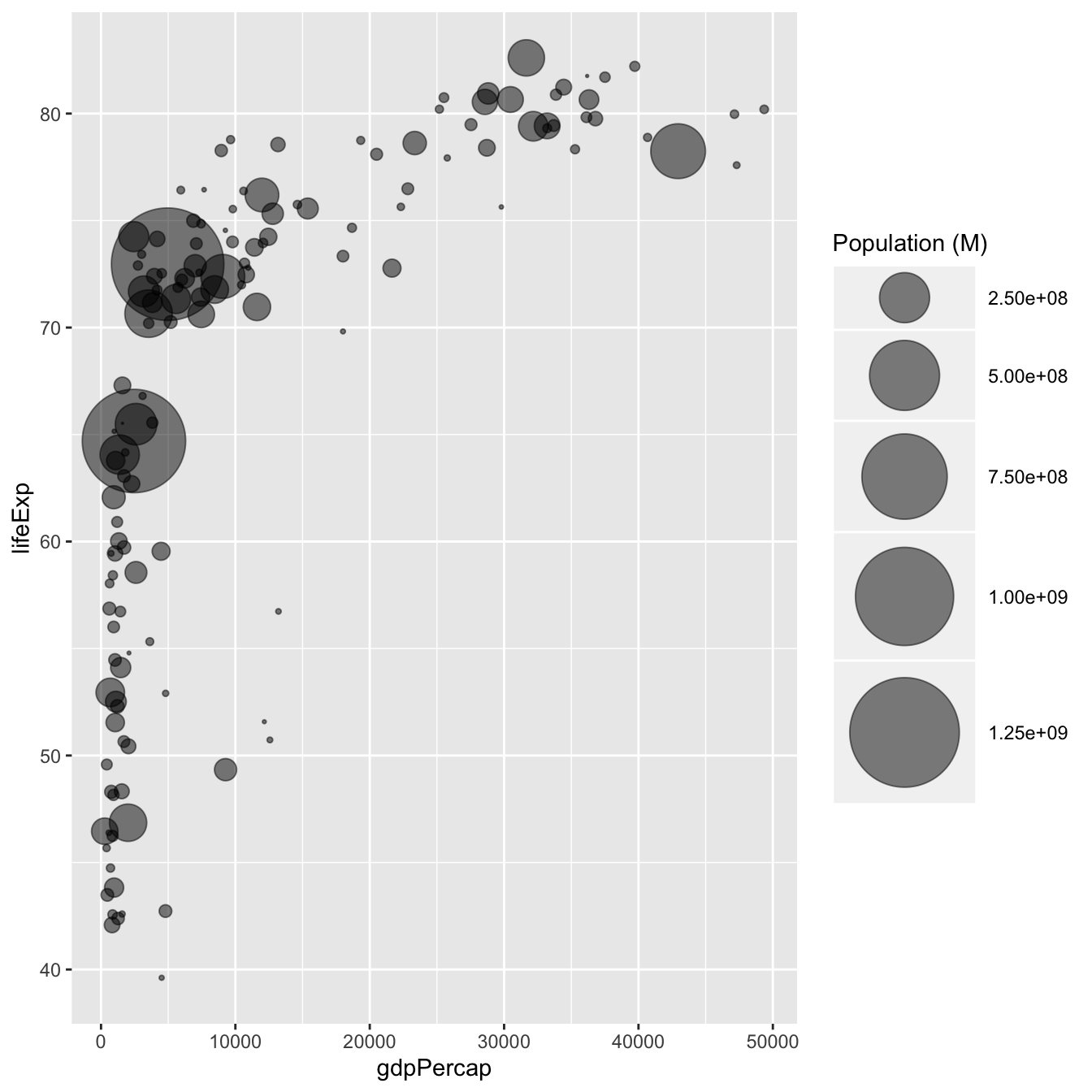

9.1.49 Add a Fourth Dimension: Color

If you have one more variable in your dataset, why not showing it using circle color? Here, the continent of each country is used to control circle color:

# Libraries
library(ggplot2)
library(dplyr)

# The dataset is provided in the gapminder library
library(gapminder)
data <- gapminder %>% filter(year=="2007") %>% dplyr::select(-year)

# Most basic bubble plot
data %>%
  arrange(desc(pop)) %>%
  mutate(country = factor(country, country)) %>%
  ggplot(aes(x=gdpPercap, y=lifeExp, size=pop, color=continent)) +
    geom_point(alpha=0.5) +
    scale_size(range = c(.1, 24), name="Population (M)")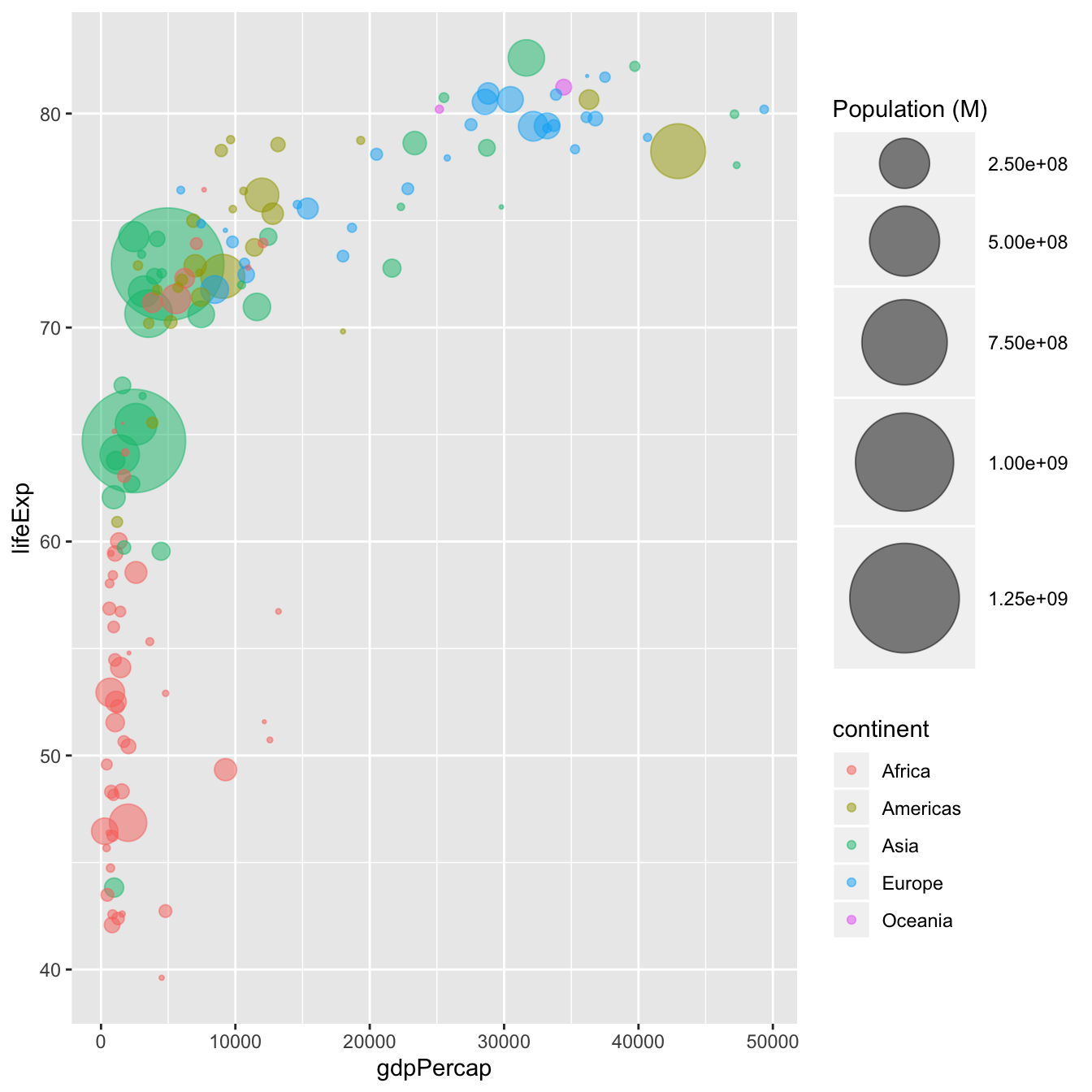

9.1.50 Make it Pretty

A few classic improvement:

• Use of the viridis package for nice color palette.
• Use of theme_ipsum() of the hrbrthemes package.
• Custom axis titles with xlab and ylab.
• Add stroke to circle: Change shape to 21 and specify color (stroke) and fill.

# Libraries
library(ggplot2)
library(dplyr)
library(hrbrthemes)
library(viridis)

# The dataset is provided in the gapminder library
library(gapminder)
data <- gapminder %>% filter(year=="2007") %>% dplyr::select(-year)

# Most basic bubble plot
data %>%
  arrange(desc(pop)) %>%
  mutate(country = factor(country, country)) %>%
  ggplot(aes(x=gdpPercap, y=lifeExp, size=pop, fill=continent)) +
    geom_point(alpha=0.5, shape=21, color="black") +
    scale_size(range = c(.1, 24), name="Population (M)") +
    scale_fill_viridis(discrete=TRUE, guide=FALSE, option="A") +
    theme_ipsum() +
    theme(legend.position="bottom") +
    ylab("Life Expectancy") +
    xlab("Gdp per Capita") +
    theme(legend.position = "none")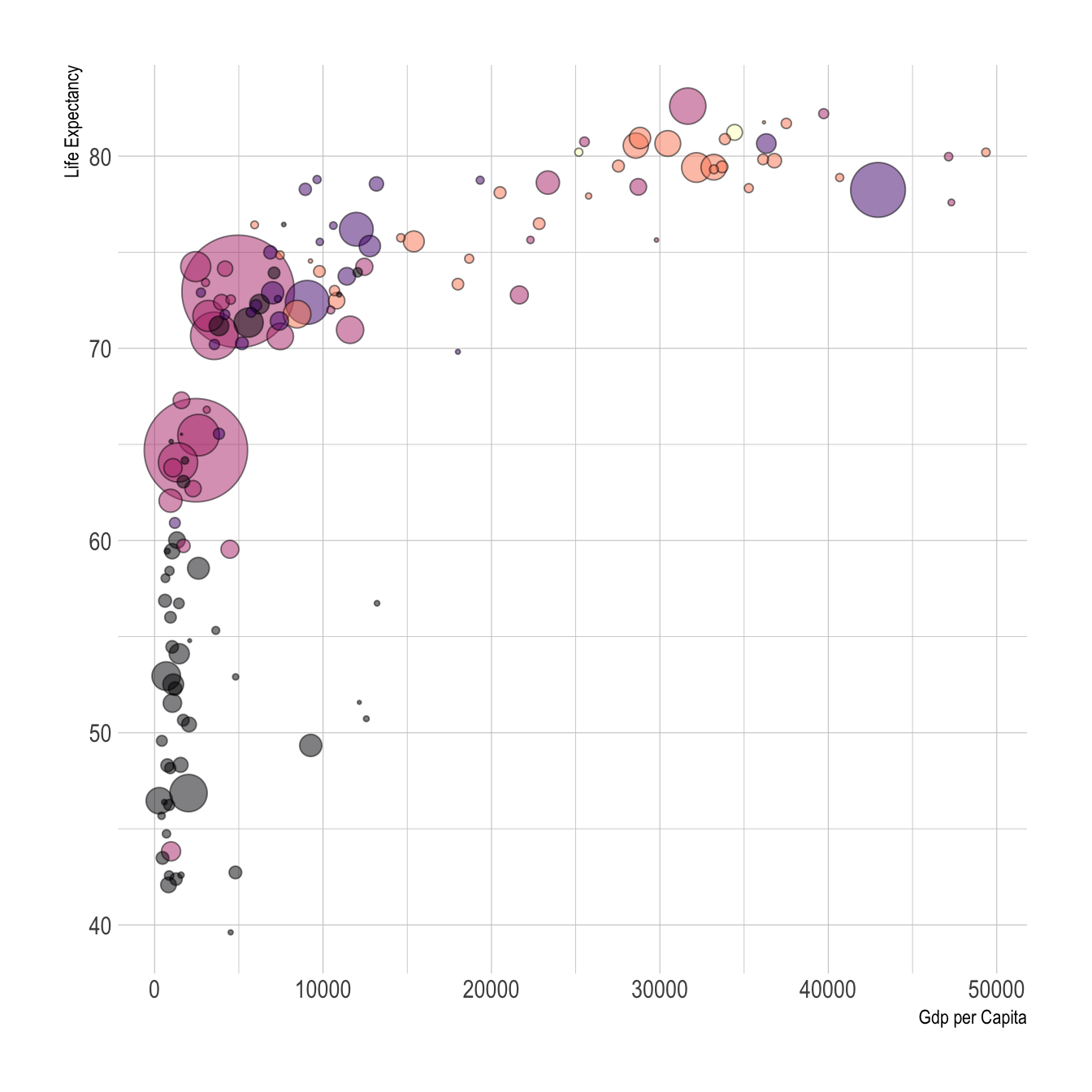

9.1.51 Connected Scatterplot with R and ggplot2

This section explains how to build a basic connected scatterplot with R and ggplot2. It provides several reproducible examples with explanation and R code.

9.1.51.1 Most Basic Connected Scatterplot: geom_point() and geom_line()

A connected scatterplot is basically a hybrid between a scatterplot and a line plot. Thus, you just have to add a geom_point() on top of the geom_line() to build it.

# Libraries
library(ggplot2)
library(dplyr)

# Load dataset from github
data <- read.table("https://raw.githubusercontent.com/holtzy/data_to_viz/master/Example_dataset/3_TwoNumOrdered.csv", header=T)
data$date <- as.Date(data$date)

# Plot
data %>%
  tail(10) %>%
  ggplot( aes(x=date, y=value)) +
    geom_line() +
    geom_point()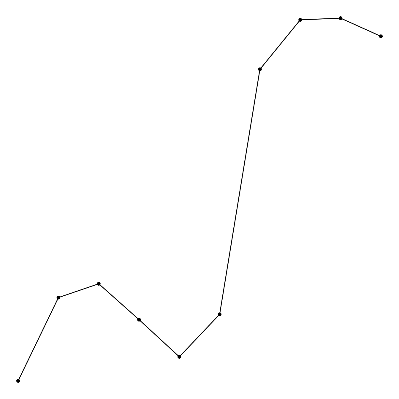

9.1.52 Customize the Connected Scatterplot

Custom the general theme with the theme_ipsum() function of the hrbrthemes package. Add a title with ggtitle(). Custom circle and line with arguments like shape, size, color and more.

# Libraries
library(ggplot2)
library(dplyr)
library(hrbrthemes)

# Load dataset from github
data <- read.table("https://raw.githubusercontent.com/holtzy/data_to_viz/master/Example_dataset/3_TwoNumOrdered.csv", header=T)
data$date <- as.Date(data$date)

# Plot
data %>%
  tail(10) %>%
  ggplot( aes(x=date, y=value)) +
    geom_line( color="grey") +
    geom_point(shape=21, color="black", fill="#69b3a2", size=6) +
    theme_ipsum() +
    ggtitle("Evolution of bitcoin price")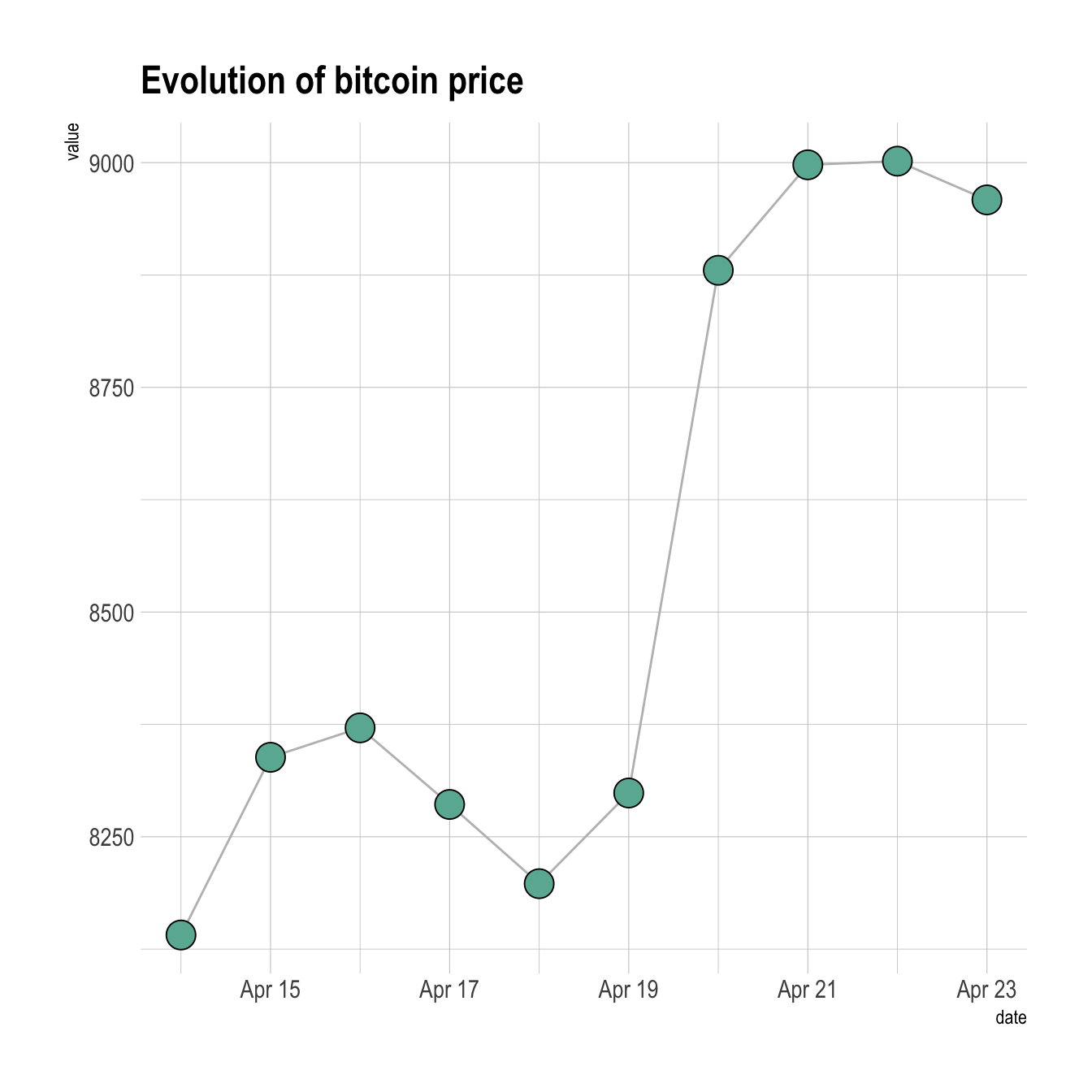

9.1.53 Connected Scatterplot to Show an Evolution

The connected scatterplot can also be a powerfull technique to tell a story about the evolution of 2 variables. Let’s consider a dataset composed of 3 columns:

• Year
• Number of baby born called Amanda this year
• Number of baby born called Ashley

The scatterplot beside allows to understand the evolution of these 2 names. Note that the code is pretty different in this case. geom_segment() is used of geom_line(). This is because geom_line() automatically sort data points depending on their X position to link them.

# Libraries
library(ggplot2)
library(dplyr)
library(babynames)
library(ggrepel)
library(tidyr)

# data
data <- babynames %>% 
  filter(name %in% c("Ashley", "Amanda")) %>%
  filter(sex=="F") %>%
  filter(year>1970) %>%
  select(year, name, n) %>%
  spread(key = name, value=n, -1)

# plot
data %>% 
  ggplot(aes(x=Amanda, y=Ashley, label=year)) +
     geom_point() +
     geom_segment(aes(
                    xend=c(tail(Amanda, n=-1), NA), 
                    yend=c(tail(Ashley, n=-1), NA)
                  )
      ) 

It makes sense to add arrows and labels to guide the reader in the chart:

# Libraries
library(ggplot2)
library(dplyr)
library(babynames)
library(ggrepel)
library(tidyr)

# data
data <- babynames %>% 
  filter(name %in% c("Ashley", "Amanda")) %>%
  filter(sex=="F") %>%
  filter(year>1970) %>%
  select(year, name, n) %>%
  spread(key = name, value=n, -1)

# Select a few date to label the chart
tmp_date <- data %>% sample_frac(0.3)

# plot 
data %>% 
  ggplot(aes(x=Amanda, y=Ashley, label=year)) +
     geom_point(color="#69b3a2") +
     geom_text_repel(data=tmp_date) +
     geom_segment(color="#69b3a2", 
                  aes(
                    xend=c(tail(Amanda, n=-1), NA), 
                    yend=c(tail(Ashley, n=-1), NA)
                  ),
                  arrow=arrow(length=unit(0.3,"cm"))
      ) +
      theme_ipsum()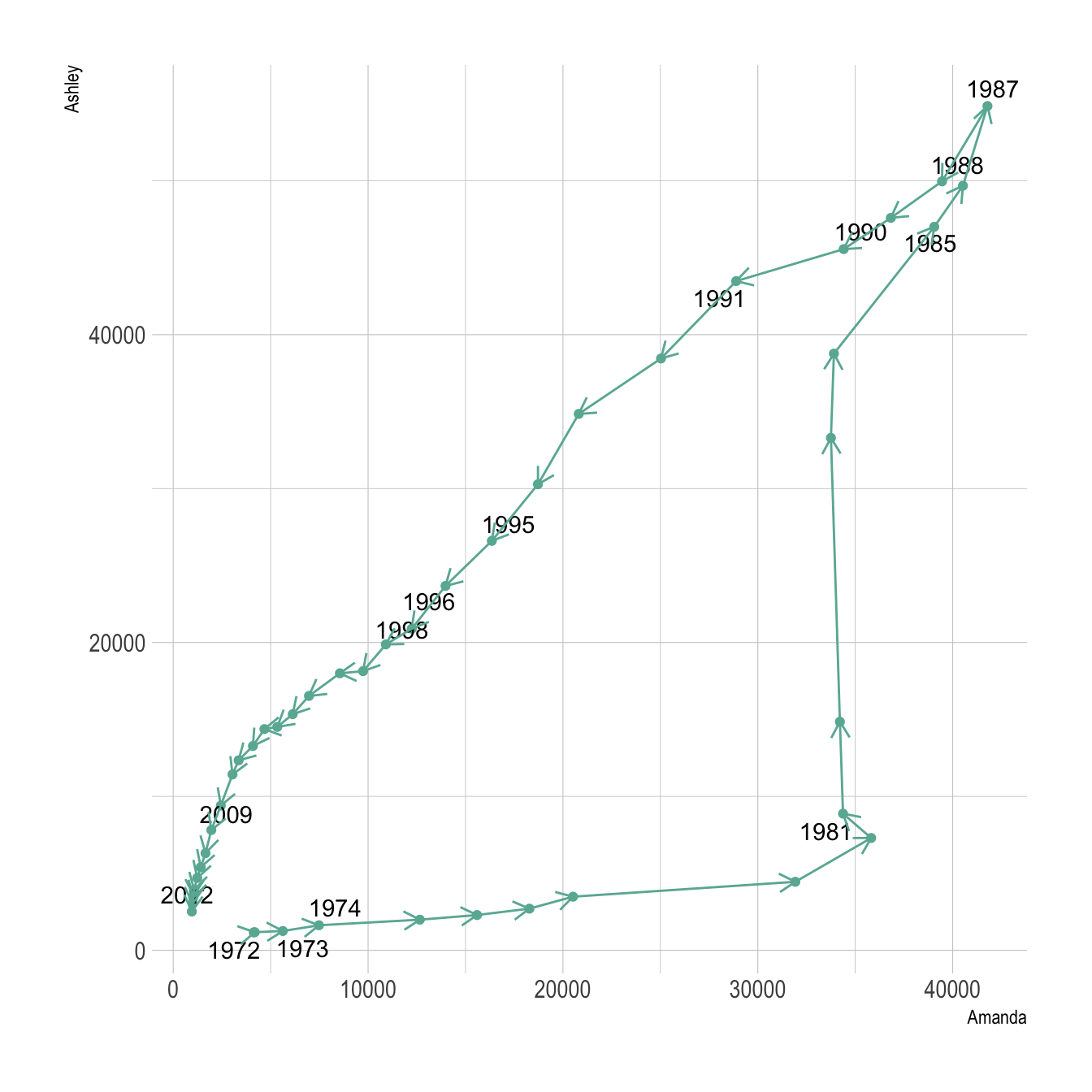

9.1.54 Parallel Coordinates Chart with ggally

ggally is a ggplot2 extension. It allows to build parallel coordinates charts thanks to the ggparcoord() function. Check several reproducible examples in this post.

9.1.54.1 Most Basic

This is the most basic parallel coordinates chart you can build with R, the ggally packages and its ggparcoord() function.

The input dataset must be a data frame with several numeric variables, each being used as a vertical axis on the chart. Columns number of these variables are specified in the columns argument of the function.

Note: here, a categoric variable is used to color lines, as specified in the groupColumn variable.

# Libraries
library(GGally)

# Data set is provided by R natively
data <- iris

# Plot
ggparcoord(data,
    columns = 1:4, groupColumn = 5
    ) 

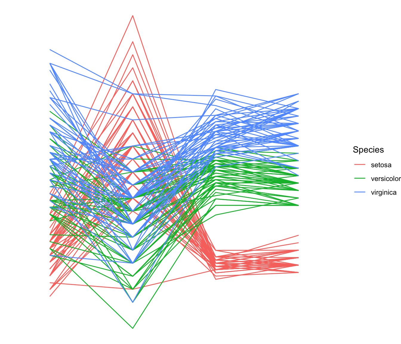
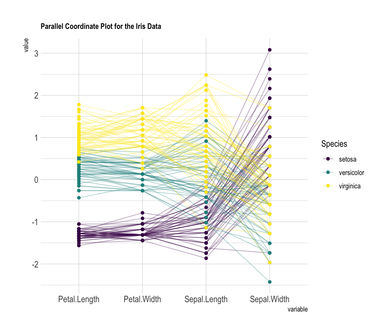
9.1.55 Custom Color, Theme, General Appearance

This is pretty much the same chart as te previous one, except for the following customizations:

• Color palette is improved thanks to the viridis package.
• Title is added with title, and customized in theme.
• Dots are added with showPoints.
• A bit of transparency is applied to lines with alphaLines.
• theme_ipsum() is used for the general appearance.

# Libraries
library(hrbrthemes)
library(GGally)
library(viridis)

# Data set is provided by R natively
data <- iris

# Plot
ggparcoord(data,
    columns = 1:4, groupColumn = 5, order = "anyClass",
    showPoints = TRUE, 
    title = "Parallel Coordinate Plot for the Iris Data",
    alphaLines = 0.3
    ) + 
  scale_color_viridis(discrete=TRUE) +
  theme_ipsum()+
  theme(
    plot.title = element_text(size=10)
  )

9.1.56 Scaling

Scaling transforms the raw data to a new scale that is common with other variables. It is a crucial step to compare variables that do not have the same unit, but can also help otherwise as shown in the example below.

The ggally package offers a scale argument. Four possible options are applied on the same dataset below:

• globalminmax - No scaling.
• uniminmax - Standardize to Min = 0 and Max = 1.
• std - Normalize univariately (substract mean & divide by sd).
• center - Standardize and center variables.

ggparcoord(data,
    columns = 1:4, groupColumn = 5, order = "anyClass",
    scale="globalminmax",
    showPoints = TRUE, 
    title = "No scaling",
    alphaLines = 0.3
    ) + 
  scale_color_viridis(discrete=TRUE) +
  theme_ipsum()+
  theme(
    legend.position="none",
    plot.title = element_text(size=13)
  ) +
  xlab("")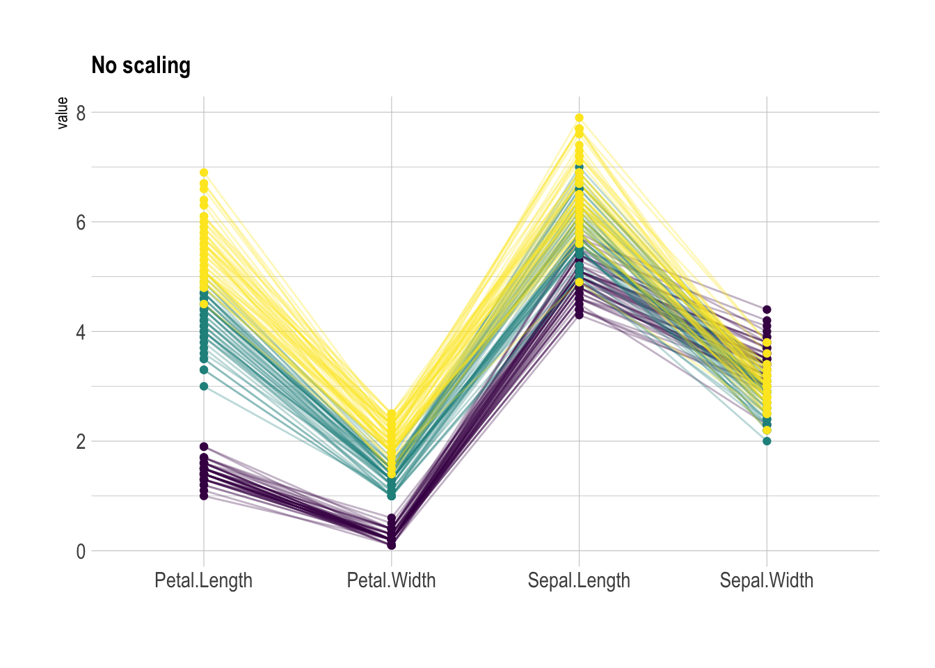

ggparcoord(data,
    columns = 1:4, groupColumn = 5, order = "anyClass",
    scale="uniminmax",
    showPoints = TRUE, 
    title = "Standardize to Min = 0 and Max = 1",
    alphaLines = 0.3
    ) + 
  scale_color_viridis(discrete=TRUE) +
  theme_ipsum()+
  theme(
    legend.position="none",
    plot.title = element_text(size=13)
  ) +
  xlab("")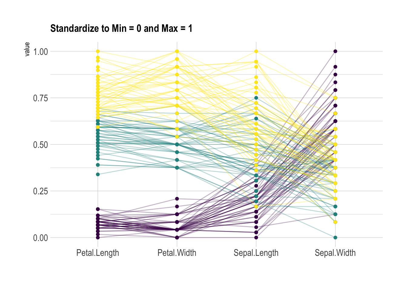

ggparcoord(data,
    columns = 1:4, groupColumn = 5, order = "anyClass",
    scale="std",
    showPoints = TRUE, 
    title = "Normalize univariately (substract mean & divide by sd)",
    alphaLines = 0.3
    ) + 
  scale_color_viridis(discrete=TRUE) +
  theme_ipsum()+
  theme(
    legend.position="none",
    plot.title = element_text(size=13)
  ) +
  xlab("")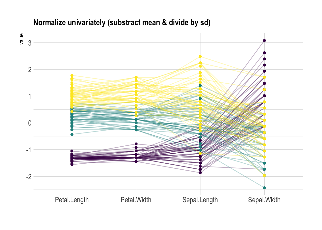

ggparcoord(data,
    columns = 1:4, groupColumn = 5, order = "anyClass",
    scale="center",
    showPoints = TRUE, 
    title = "Standardize and center variables",
    alphaLines = 0.3
    ) + 
  scale_color_viridis(discrete=TRUE) +
  theme_ipsum()+
  theme(
    legend.position="none",
    plot.title = element_text(size=13)
  ) +
  xlab("")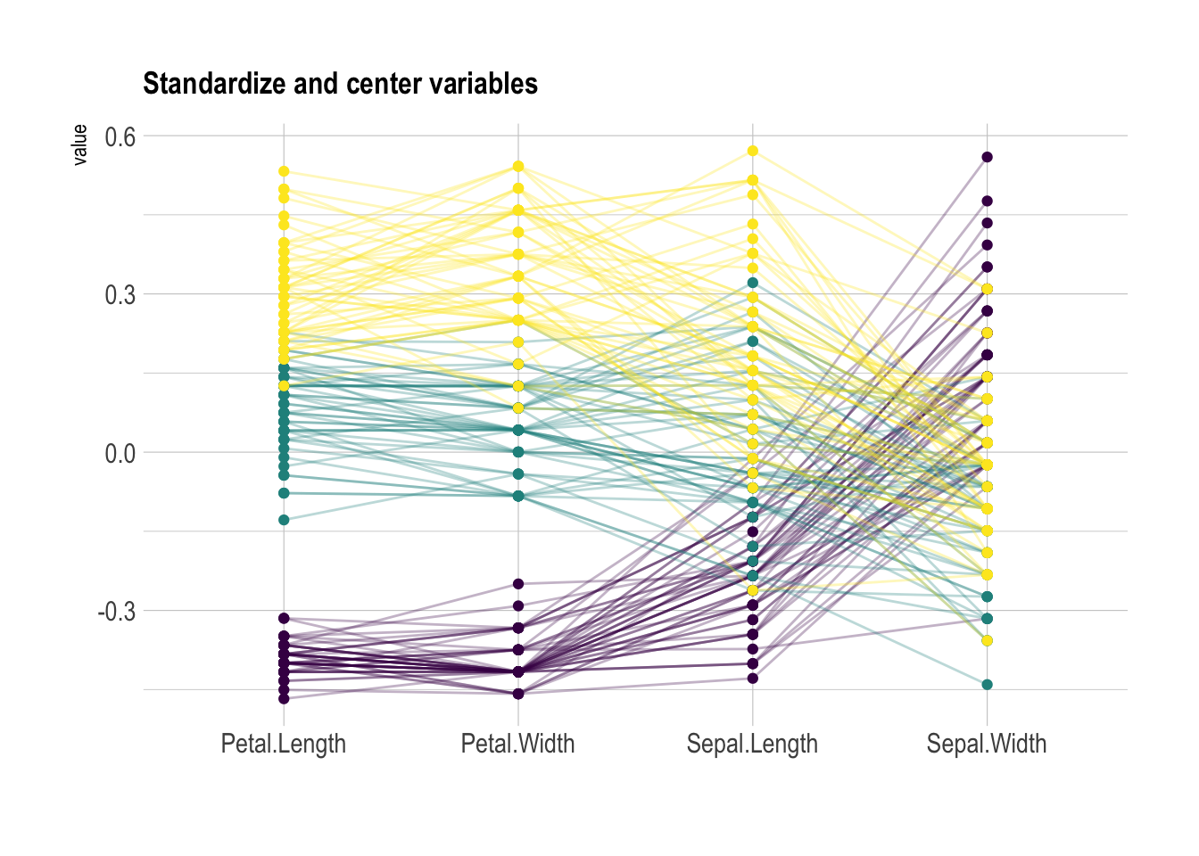

9.1.57 Highlight a Group

Data visualization aims to highlight a story in the data. If you are interested in a specific group, you can highlight it as follow:

# Libraries
library(GGally)
library(dplyr)

# Data set is provided by R natively
data <- iris

# Plot
data %>%
  arrange(desc(Species)) %>%
  ggparcoord(
    columns = 1:4, groupColumn = 5, order = "anyClass",
    showPoints = TRUE, 
    title = "Original",
    alphaLines = 1
    ) + 
  scale_color_manual(values=c( "#69b3a2", "#E8E8E8", "#E8E8E8") ) +
  theme_ipsum()+
  theme(
    legend.position="Default",
    plot.title = element_text(size=10)
  ) +
  xlab("")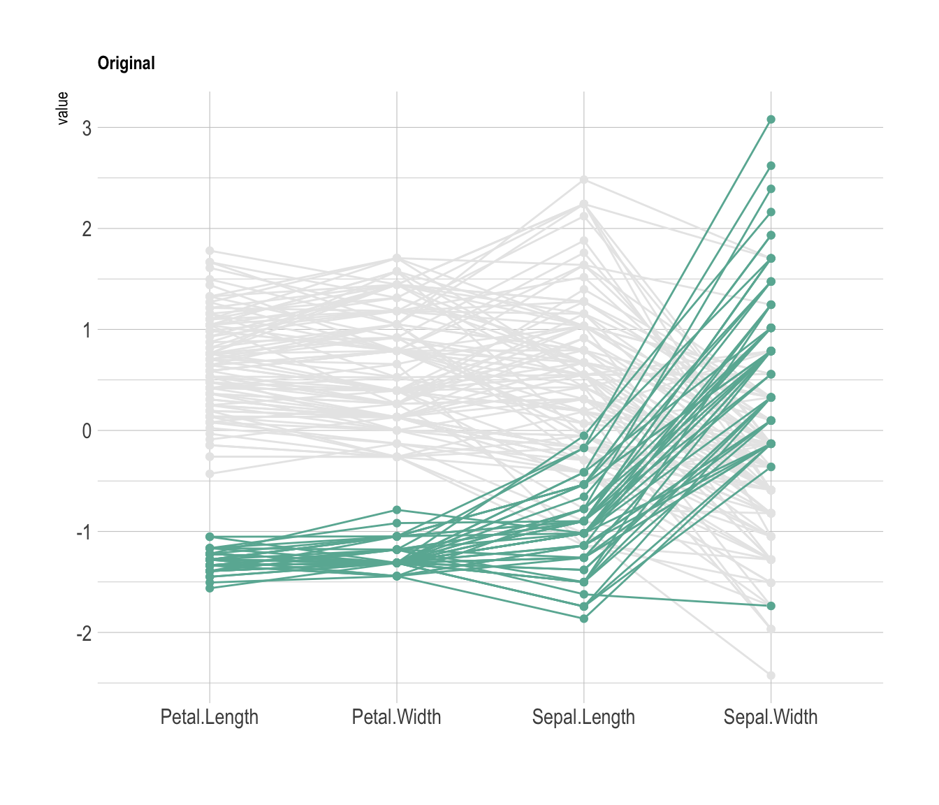

9.1.58 Lollipop Chart with Conditional Color

If your lollipop plot goes on both side of an interesting threshold, you probably want to change the color of its components conditionally. Here is how using R and ggplot2.

9.1.59 Marker

Here is the process to use conditional color on your ggplot2 chart:

• Add a new column to your dataframe specifying if you are over or under the threshold (use an ifelse statement).
• Give this column to the color aesthetic.

# library
library(ggplot2)
library(dplyr)

# Create data (this takes more sense with a numerical X axis)
x <- seq(0, 2*pi, length.out=100)
data <- data.frame(
  x=x, 
  y=sin(x) + rnorm(100, sd=0.2)
)
 
# Add a column with your condition for the color
data <- data %>% 
  mutate(mycolor = ifelse(y>0, "type1", "type2"))
 
# plot
ggplot(data, aes(x=x, y=y)) +
  geom_segment( aes(x=x, xend=x, y=0, yend=y, color=mycolor), size=1.3, alpha=0.9) +
  theme_light() +
  theme(
    legend.position = "none",
    panel.border = element_blank(),
  ) +
  xlab("") +
  ylab("Value of Y")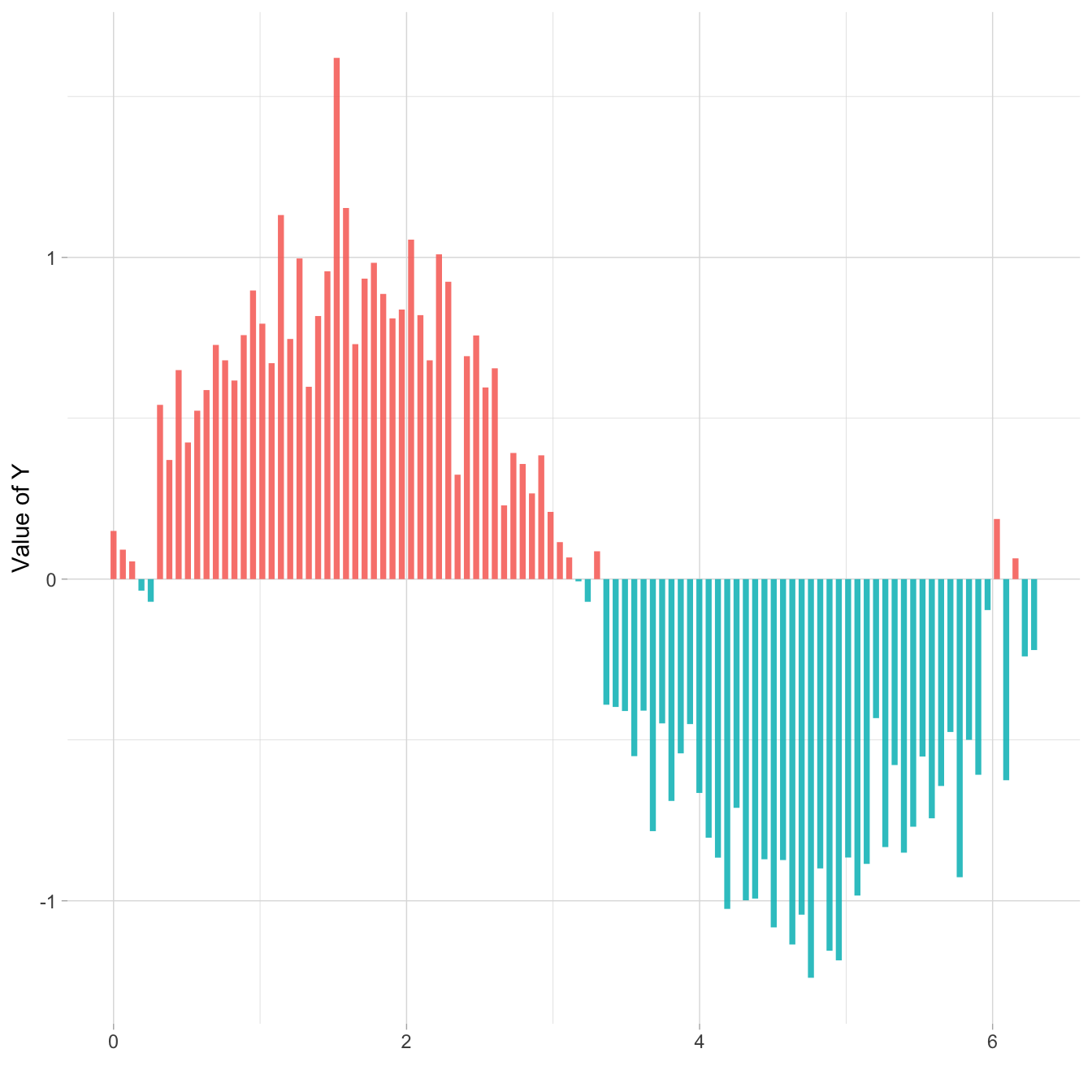

9.1.60 Lollipop Chart with 2 Groups

A lollipop chart can be used to compare 2 categories, linking them with a segment to stress out their difference. This post explains how to do it with R and ggplot2.

Lollipop plots can be very appropriate when it comes to compare 2 values for several entities.

For each entity, one point is drawn for each variable, with a different color. Their difference is then highlighted using a segment. This type of visualisation is also called Cleveland dot plots.

As usual, it is advised to order your individuals by mean, median, or group difference to give even more insight to the figure.

# Library
library(ggplot2)
library(dplyr)
library(hrbrthemes)

# Create data
value1 <- abs(rnorm(26))*2
data <- data.frame(
  x=LETTERS[1:26], 
  value1=value1, 
  value2=value1+1+rnorm(26, sd=1) 
)
 
# Reorder data using average? Learn more about reordering in chart #267
data <- data %>% 
  rowwise() %>% 
  mutate( mymean = mean(c(value1,value2) )) %>% 
  arrange(mymean) %>% 
  mutate(x=factor(x, x))
 
# Plot
ggplot(data) +
  geom_segment( aes(x=x, xend=x, y=value1, yend=value2), color="grey") +
  geom_point( aes(x=x, y=value1), color=rgb(0.2,0.7,0.1,0.5), size=3 ) +
  geom_point( aes(x=x, y=value2), color=rgb(0.7,0.2,0.1,0.5), size=3 ) +
  coord_flip()+
  theme_ipsum() +
  theme(
    legend.position = "none",
  ) +
  xlab("") +
  ylab("Value of Y")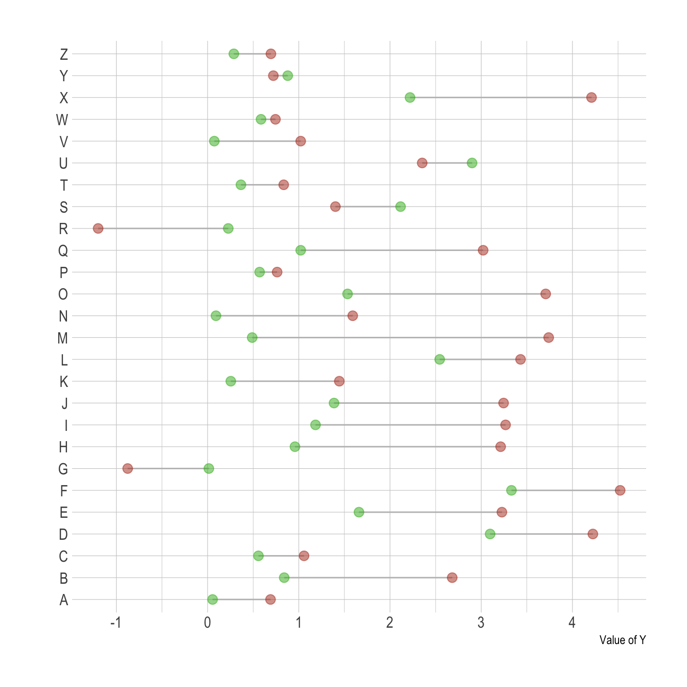

9.1.61 Circular Barplot with Groups

This section explains how to build a circular barchart with groups. A gap is added between groups to highlight them. Bars are labeled, group names are annotated

9.1.62 Add a Gap in the Circle

A circular barplot is a barplot where bars are displayed along a circle instead of a line. This page aims to teach you how to make a circular barplot with groups.

Since this kind of chart is a bit tricky, I strongly advise to understand graph #295 and #296 that will teach you the basics.

The first step is to build a circular barplot with a break in the circle. Actually, I just added a few empty lines at the end of the initial data frame:

# library
library(tidyverse)
 
# Create dataset
data <- data.frame(
  individual=paste( "Mister ", seq(1,60), sep=""),
  value=sample( seq(10,100), 60, replace=T)
)
 
# Set a number of 'empty bar'
empty_bar <- 10
 
# Add lines to the initial dataset
to_add <- matrix(NA, empty_bar, ncol(data))
colnames(to_add) <- colnames(data)
data <- rbind(data, to_add)
data$id <- seq(1, nrow(data))
 
# Get the name and the y position of each label
label_data <- data
number_of_bar <- nrow(label_data)
angle <- 90 - 360 * (label_data$id-0.5) /number_of_bar     # I substract 0.5 because the letter must have the angle of the center of the bars. Not extreme right(1) or extreme left (0)
label_data$hjust <- ifelse( angle < -90, 1, 0)
label_data$angle <- ifelse(angle < -90, angle+180, angle)
 
# Make the plot
p <- ggplot(data, aes(x=as.factor(id), y=value)) +       # Note that id is a factor. If x is numeric, there is some space between the first bar
  geom_bar(stat="identity", fill=alpha("green", 0.3)) +
  ylim(-100,120) +
  theme_minimal() +
  theme(
    axis.text = element_blank(),
    axis.title = element_blank(),
    panel.grid = element_blank(),
    plot.margin = unit(rep(-1,4), "cm") 
  ) +
  coord_polar(start = 0) + 
  geom_text(data=label_data, aes(x=id, y=value+10, label=individual, hjust=hjust), color="black", fontface="bold",alpha=0.6, size=2.5, angle= label_data$angle, inherit.aes = FALSE ) 
 
p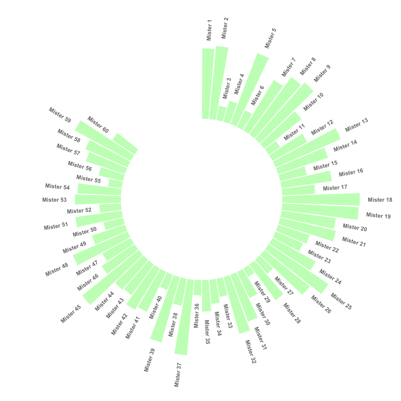

9.1.63 Space between Groups

This concept can now be used to add space between each group of the dataset. I add n lines with only NA at the bottom of each group.

This chart is far more insightful since it allows one to quickly compare the different groups, and to compare the value of items within each group.

# library
library(tidyverse)
 
# Create dataset
data <- data.frame(
  individual=paste( "Mister ", seq(1,60), sep=""),
  group=c( rep('A', 10), rep('B', 30), rep('C', 14), rep('D', 6)) ,
  value=sample( seq(10,100), 60, replace=T)
)
 
# Set a number of 'empty bar' to add at the end of each group
empty_bar <- 4
to_add <- data.frame( matrix(NA, empty_bar*nlevels(data$group), ncol(data)) )
colnames(to_add) <- colnames(data)
to_add$group <- rep(levels(data$group), each=empty_bar)
data <- rbind(data, to_add)
data <- data %>% arrange(group)
data$id <- seq(1, nrow(data))
 
# Get the name and the y position of each label
label_data <- data
number_of_bar <- nrow(label_data)
angle <- 90 - 360 * (label_data$id-0.5) /number_of_bar     # I substract 0.5 because the letter must have the angle of the center of the bars. Not extreme right(1) or extreme left (0)
label_data$hjust <- ifelse( angle < -90, 1, 0)
label_data$angle <- ifelse(angle < -90, angle+180, angle)
 
# Make the plot
p <- ggplot(data, aes(x=as.factor(id), y=value, fill=group)) +       # Note that id is a factor. If x is numeric, there is some space between the first bar
  geom_bar(stat="identity", alpha=0.5) +
  ylim(-100,120) +
  theme_minimal() +
  theme(
    legend.position = "none",
    axis.text = element_blank(),
    axis.title = element_blank(),
    panel.grid = element_blank(),
    plot.margin = unit(rep(-1,4), "cm") 
  ) +
  coord_polar() + 
  geom_text(data=label_data, aes(x=id, y=value+10, label=individual, hjust=hjust), color="black", fontface="bold",alpha=0.6, size=2.5, angle= label_data$angle, inherit.aes = FALSE ) 
 
p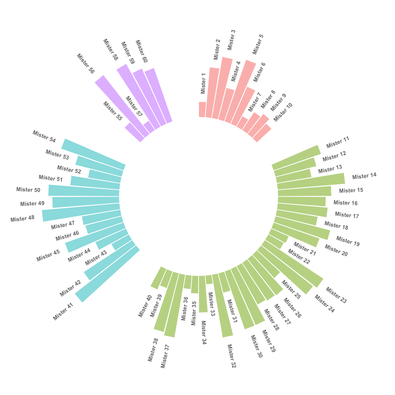

9.1.64 Order Bars

Here observations are sorted by bar height within each group. It can be useful if your goal is to understand what are the highest / lowest observations within and across groups.

The method used to order groups in ggplot2 is extensively described in this dedicated page. Basically, you just have to add the following piece of code right after the data frame creation:

# Order data:
data = data %>% arrange(group, value)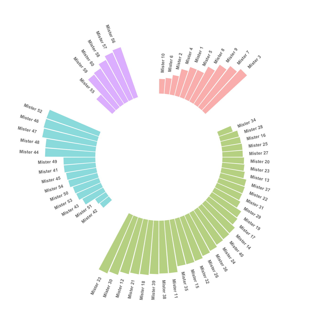

9.1.65 Circular Barchart Customization

Last but not least, it is highly advisable to add some customisation to your chart. Here we add group names (A, B, C and D), and we add a scale to help compare the sizes of the bars. Voila! The code is a bit long, but the result is quite worth it in my opinion!

# library
library(tidyverse)
 
# Create dataset
data <- data.frame(
  individual=paste( "Mister ", seq(1,60), sep=""),
  group=c( rep('A', 10), rep('B', 30), rep('C', 14), rep('D', 6)) ,
  value=sample( seq(10,100), 60, replace=T)
)
 
# Set a number of 'empty bar' to add at the end of each group
empty_bar <- 3
to_add <- data.frame( matrix(NA, empty_bar*nlevels(data$group), ncol(data)) )
colnames(to_add) <- colnames(data)
to_add$group <- rep(levels(data$group), each=empty_bar)
data <- rbind(data, to_add)
data <- data %>% arrange(group)
data$id <- seq(1, nrow(data))
 
# Get the name and the y position of each label
label_data <- data
number_of_bar <- nrow(label_data)
angle <- 90 - 360 * (label_data$id-0.5) /number_of_bar     # I substract 0.5 because the letter must have the angle of the center of the bars. Not extreme right(1) or extreme left (0)
label_data$hjust <- ifelse( angle < -90, 1, 0)
label_data$angle <- ifelse(angle < -90, angle+180, angle)
 
# prepare a data frame for base lines
base_data <- data %>% 
  group_by(group) %>% 
  summarize(start=min(id), end=max(id) - empty_bar) %>% 
  rowwise() %>% 
  mutate(title=mean(c(start, end)))
 
# prepare a data frame for grid (scales)
grid_data <- base_data
grid_data$end <- grid_data$end[ c( nrow(grid_data), 1:nrow(grid_data)-1)] + 1
grid_data$start <- grid_data$start - 1
grid_data <- grid_data[-1,]
 
# Make the plot
p <- ggplot(data, aes(x=as.factor(id), y=value, fill=group)) +       # Note that id is a factor. If x is numeric, there is some space between the first bar
  
  geom_bar(aes(x=as.factor(id), y=value, fill=group), stat="identity", alpha=0.5) +
  
  # Add a val=100/75/50/25 lines. I do it at the beginning to make sur barplots are OVER it.
  geom_segment(data=grid_data, aes(x = end, y = 80, xend = start, yend = 80), colour = "grey", alpha=1, size=0.3 , inherit.aes = FALSE ) +
  geom_segment(data=grid_data, aes(x = end, y = 60, xend = start, yend = 60), colour = "grey", alpha=1, size=0.3 , inherit.aes = FALSE ) +
  geom_segment(data=grid_data, aes(x = end, y = 40, xend = start, yend = 40), colour = "grey", alpha=1, size=0.3 , inherit.aes = FALSE ) +
  geom_segment(data=grid_data, aes(x = end, y = 20, xend = start, yend = 20), colour = "grey", alpha=1, size=0.3 , inherit.aes = FALSE ) +
  
  # Add text showing the value of each 100/75/50/25 lines
  annotate("text", x = rep(max(data$id),4), y = c(20, 40, 60, 80), label = c("20", "40", "60", "80") , color="grey", size=3 , angle=0, fontface="bold", hjust=1) +
  
  geom_bar(aes(x=as.factor(id), y=value, fill=group), stat="identity", alpha=0.5) +
  ylim(-100,120) +
  theme_minimal() +
  theme(
    legend.position = "none",
    axis.text = element_blank(),
    axis.title = element_blank(),
    panel.grid = element_blank(),
    plot.margin = unit(rep(-1,4), "cm") 
  ) +
  coord_polar() + 
  geom_text(data=label_data, aes(x=id, y=value+10, label=individual, hjust=hjust), color="black", fontface="bold",alpha=0.6, size=2.5, angle= label_data$angle, inherit.aes = FALSE ) +
  
  # Add base line information
  geom_segment(data=base_data, aes(x = start, y = -5, xend = end, yend = -5), colour = "black", alpha=0.8, size=0.6 , inherit.aes = FALSE )  +
  geom_text(data=base_data, aes(x = title, y = -18, label=group), hjust=c(1,1,0,0), colour = "black", alpha=0.8, size=4, fontface="bold", inherit.aes = FALSE)
 
p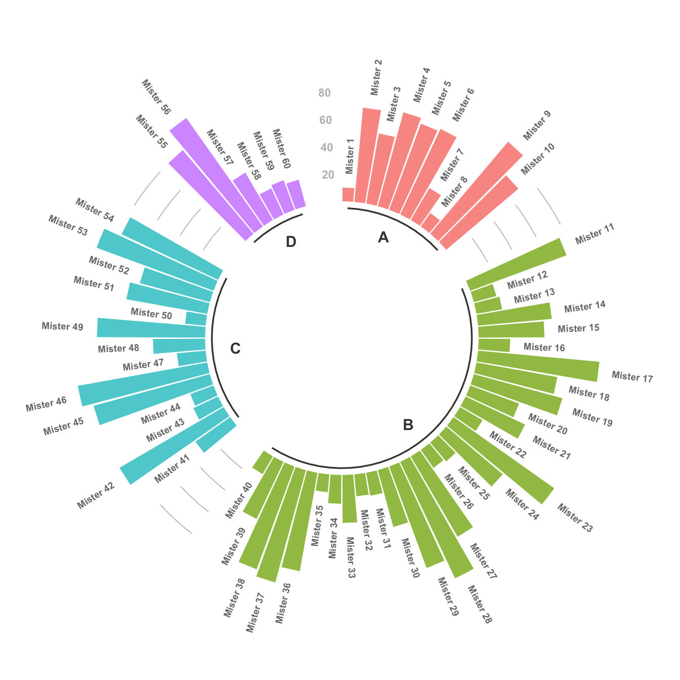

{85%}

9.1.66 What is Stacking

Stacking is a process where a chart is broken up across more than one categoric variables which make up the whole. Each item of the categoric variable is represented by a shaded area. These areas are stacked on top of one another.

Here is an example with a stacked area chart. It shows the evolution of baby name occurence in the US between 1880 and 2015. Six first names are represented on top of one another.

# Libraries
library(tidyverse)
library(babynames)
library(streamgraph)
library(viridis)
library(hrbrthemes)
library(plotly)

# Load dataset from github
data <- babynames %>% 
  filter(name %in% c("Amanda", "Jessica",    "Patricia", "Deborah",   "Dorothy",  "Helen")) %>%
  filter(sex=="F")

# Plot
p <- data %>% 
  ggplot( aes(x=year, y=n, fill=name, text=name)) +
    geom_area( ) +
    scale_fill_viridis(discrete = TRUE) +
    theme(legend.position="none") +
    ggtitle("Popularity of American names in the previous 30 years") +
    theme_ipsum() +
    theme(legend.position="none")
ggplotly(p, tooltip="text")

9.1.67 Example: Optical Illusion

Important note: this section is inspired from this post by Dr. Drang.

Dr Drang gives this nice example. Consider the graphic below, and try to visualize how the 3 categories evolved on the period:

# create dummy data
don <- data.frame(
  x = rep(seq(2000,2005), 3),
  value = c(  75, 73, 68, 57, 36, 0, 15, 16, 17, 18, 19, 20, 10, 11, 15, 25, 45, 80),
  group = rep(c("A", "B", "C"), each=6)
)

#plot
don %>% 
  ggplot( aes(x=x, y=value, fill=group)) +
    geom_area( ) +
    scale_fill_viridis(discrete = TRUE) +
    theme(legend.position="none") +
    theme_ipsum() +
    theme(legend.position="none")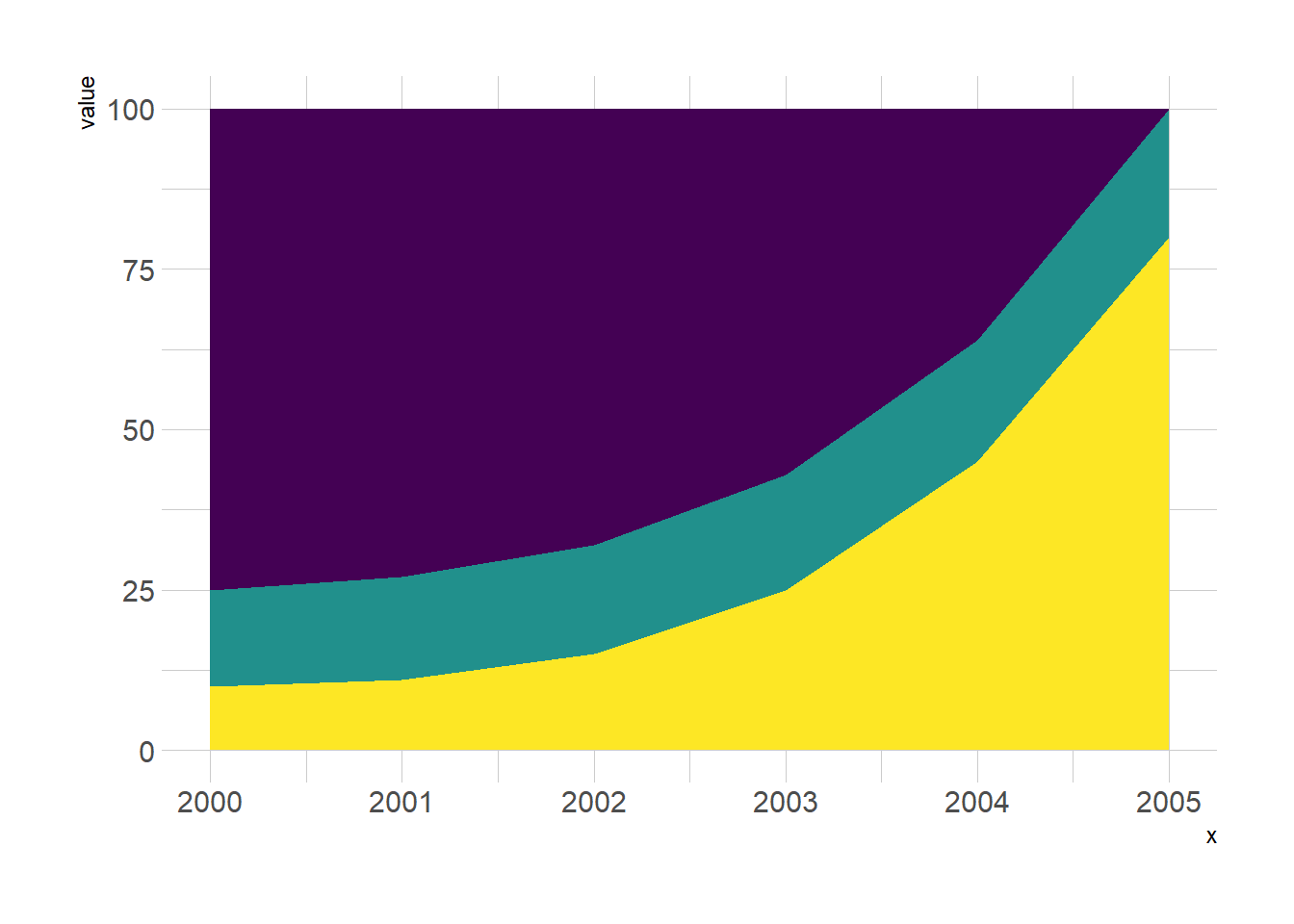

It looks obvious that the yellow category increased, the purple decreased, and the green. is harder to read. At a first glance it looks like it is slightly decreasing I would say.

Now let’s plot just the green group to find out:

#plot
don %>% 
  filter(group=="B") %>%
  ggplot( aes(x=x, y=value, fill=group)) +
    geom_area( fill="#22908C") +
    theme(legend.position="none") +
    theme_ipsum() +
    theme(legend.position="none")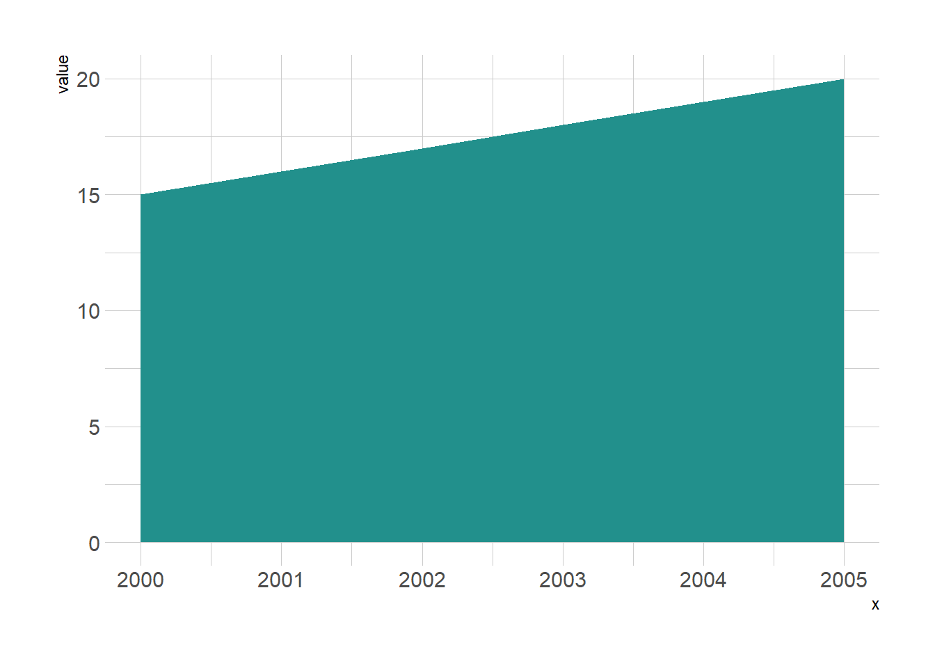

9.1.68 Workaround

If you have just a few categories, I would suggest to build a line chart. Here it is easy to follow a category and understand how it evolved accurately.

data %>%
  ggplot( aes(x=year, y=n, group=name, color=name)) +
    geom_line() +
    scale_color_viridis(discrete = TRUE) +
    theme(legend.position="none") +
    ggtitle("Popularity of American names in the previous 30 years") +
    theme_ipsum()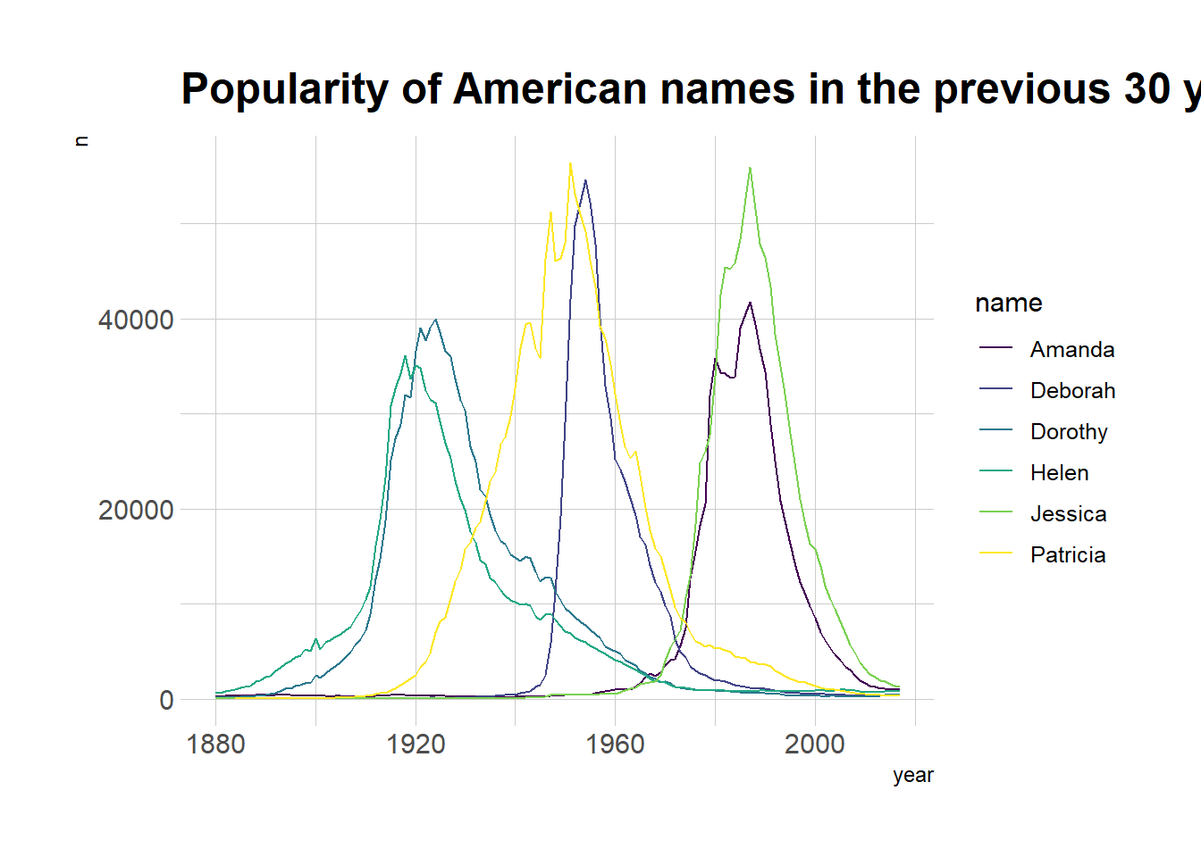

However, this solution is not suitable if you have many categories. Indeed, it would result in a spaghetti chart that is very hard to read. You can read more about this here.

Instead I would suggest to use `small multiple: here each category has its own section in the graphic. It makes easy to understand the pattern of each category.

data %>%
  ggplot( aes(x=year, y=n, group=name, fill=name)) +
    geom_area() +
    scale_fill_viridis(discrete = TRUE) +
    theme(legend.position="none") +
    ggtitle("Popularity of American names in the previous 30 years") +
    theme_ipsum() +
    theme(
      legend.position="none",
      panel.spacing = unit(0.1, "lines"),
      strip.text.x = element_text(size = 8)
    ) +
    facet_wrap(~name, scale="free_y")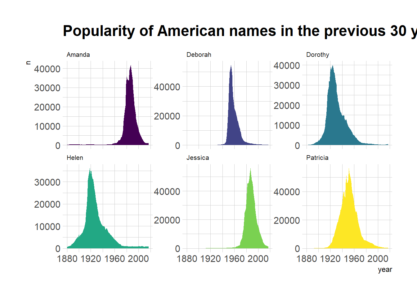

9.1.69 Basic Stacked area Chart with R

This section provides the basics concerning stacked area chart with R and ggplot2. It takes into account several input format types and show how to customize the output.

9.1.70 Most Basic Stacked Area with ggplot2

The data frame used as input to build a stacked area chart requires 3 columns:

• x: numeric variable used for the X axis, often it is a time.
• y: numeric variable used for the Y axis. What are we looking at?
• group: one shape will be done per group.

The chart is built using the geom_area() function.

# Packages
library(ggplot2)
library(dplyr)
 
# create data
time <- as.numeric(rep(seq(1,7),each=7))  # x Axis
value <- runif(49, 10, 100)               # y Axis
group <- rep(LETTERS[1:7],times=7)        # group, one shape per group
data <- data.frame(time, value, group)

# stacked area chart
ggplot(data, aes(x=time, y=value, fill=group)) + 
    geom_area()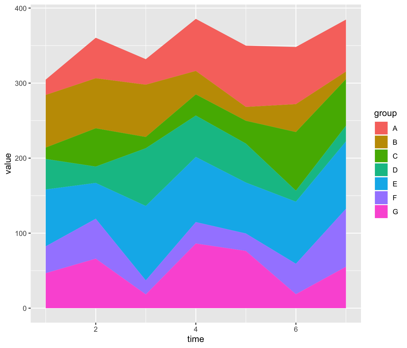

9.1.71 Control Stacking Order with ggplot2

The gallery offers a post dedicated to reordering with ggplot2. This step can be tricky but the code below shows how to:

• Give a specific order with the factor() function.
• Order alphabetically using sort().
• Order following values at a specific data.

# Give a specific order:
data$group <- factor(data$group , levels=c("B", "A", "D", "E", "G", "F", "C") )

# Plot again
ggplot(data, aes(x=time, y=value, fill=group)) + 
    geom_area()

# Note: you can also sort levels alphabetically:
myLevels <- levels(data$group)
data$group <- factor(data$group , levels=sort(myLevels) )

# Note: sort followinig values at time = 5
myLevels <- data %>%
  filter(time==6) %>%
  arrange(value)
data$group <- factor(data$group , levels=myLevels$group )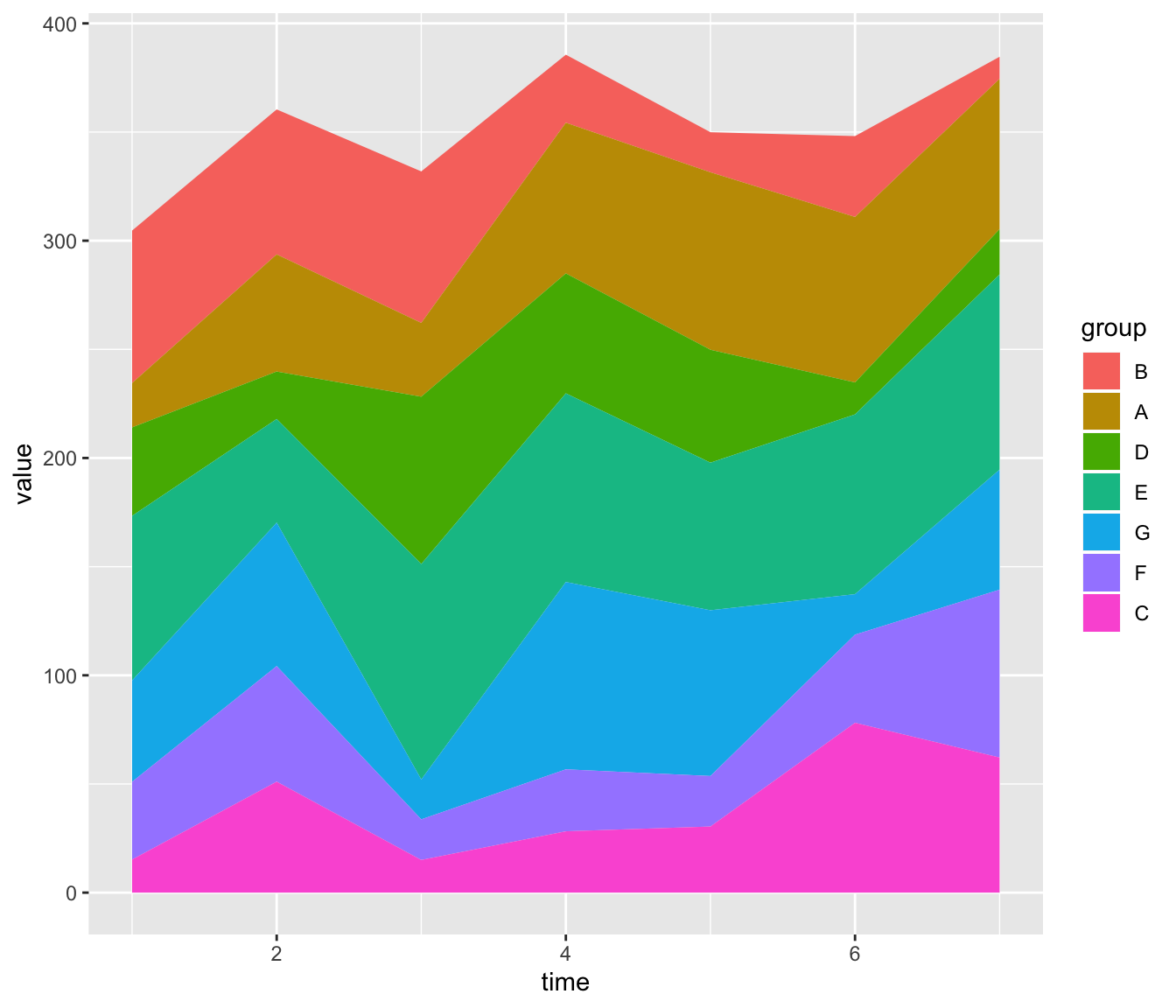

9.1.72 Proportional Stacked Area Chart

In a proportional stacked area graph, the sum of each year is always equal to hundred and value of each group is represented through percentages.

To make it, you have to calculate these percentages first. This can be done using dplyr of with base R.

# Compute percentages with dplyr
library(dplyr)
data <- data  %>%
  group_by(time, group) %>%
  summarise(n = sum(value)) %>%
  mutate(percentage = n / sum(n))

# Plot
ggplot(data, aes(x=time, y=percentage, fill=group)) + 
    geom_area(alpha=0.6 , size=1, colour="black")

# Note: compute percentages without dplyr:
my_fun <- function(vec){ 
  as.numeric(vec[2]) / sum(data$value[data$time==vec[1]]) *100 
}
data$percentage <- apply(data , 1 , my_fun)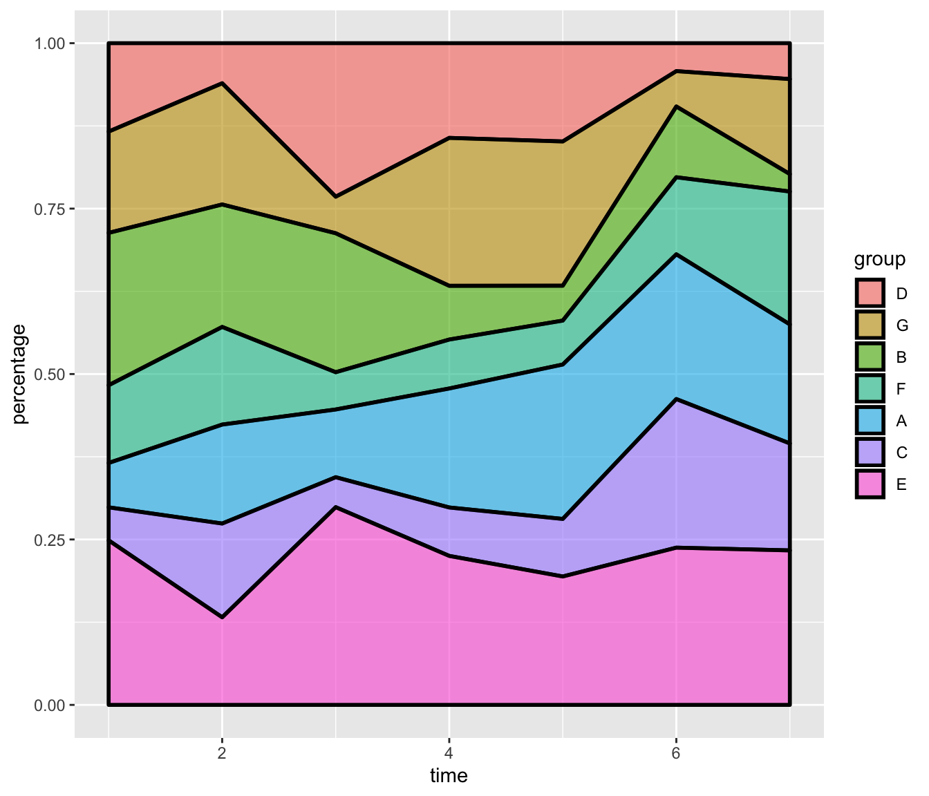

9.1.73 Color & Style

Let’s improve the chart general appearance:

• Usage of the viridis color scale.
• theme_ipsum of the hrbrthemes package.
• Add title with ggtitle.

# Library
library(viridis)
library(hrbrthemes)

# Plot
ggplot(data, aes(x=time, y=value, fill=group)) + 
    geom_area(alpha=0.6 , size=.5, colour="white") +
    scale_fill_viridis(discrete = T) +
    theme_ipsum() + 
    ggtitle("The race between ...")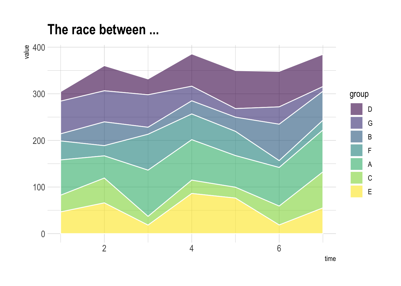

9.2 Data Art

Sometimes programming can be used to generate figures that are aestetically pleasing, but don’t bring any insight. Here are a few pieces of data art built from R and ggplot2. Visit data-to-art.com for more.

9.2.1 Using R and ggplot2 for Data Art.

R and ggplot2 are awesome tool to produce random shapes. Welcome in the field of generative coding or data art.

set.seed(345)
library(ggplot2)
library(RColorBrewer)
ngroup=30
names=paste("G_",seq(1,ngroup),sep="")
DAT=data.frame()

for(i in seq(1:30)){
    data=data.frame( matrix(0, ngroup , 3))
    data[,1]=i
    data[,2]=sample(names, nrow(data))
    data[,3]=prop.table(sample( c(rep(0,100),c(1:ngroup)) ,nrow(data)))
    DAT=rbind(DAT,data)
    }
colnames(DAT)=c("Year","Group","Value")
DAT=DAT[order( DAT$Year, DAT$Group) , ]


coul = brewer.pal(12, "Paired") 
coul = colorRampPalette(coul)(ngroup)
coul=coul[sample(c(1:length(coul)) , size=length(coul) ) ]

ggplot(DAT, aes(x=Year, y=Value, fill=Group )) + 
    geom_area(alpha=1  )+
    theme_bw() +
    #scale_fill_brewer(colour="red", breaks=rev(levels(DAT$Group)))+
    scale_fill_manual(values = coul)+
     theme(
        text = element_blank(),
        line = element_blank(),
        title = element_blank(),
        legend.position="none",
        panel.border = element_blank(),
        panel.background = element_blank())

9.2.2 R Snail

A piece of generative art built by Christophe Cariou with R.

par(mfrow=c(1,1),mar=c(0,0,0,0),oma=c(1,1,1,1))
plot(0,0,type="n", xlim=c(-2,32), ylim=c(3,27),
    xaxs="i", yaxs="i", axes=FALSE, xlab=NA, ylab=NA,
    asp=1)

for (j in 0:35) {
for (i in 0:35) {

    R <- 8
    alpha <- j*10
    X <- 15+R*cos(alpha/180*pi)
    Y <- 15+R*sin(alpha/180*pi)

    r <- 3
    beta <- i*10
    x <- 15+r*cos(beta/180*pi)
    y <- 15+r*sin(beta/180*pi)

    d1 <- sqrt((X-x)^2+(Y-y)^2)
    xc <- x
    yc <- y

  n <- 180-atan((Y-y)/(X-x))/pi*180

    alpha2 <- -(0:n)
    theta <- alpha2/180*pi

    b <- d1/(n/180*pi)
    r <- b*theta

    x1 <- xc+r*cos(theta)
    y1 <- yc+r*sin(theta)

    lines(x1,y1, col="black")

    }
}

9.3 Animation

An animated chart displays several chart states one after the other.

It must not be confounded with an interactive chart that allows interaction like zooming or hovering. This section describes 2 methods to build animations with R.

The first method builds many png images and concatenate them in a gif using image magick. The second relies on the gganimate package that automatically builds the animation for you.

Here is a great interactive course that helps getting started with animations.

9.3.0.1 Build-Animation Directly with gganimate

The gganimate library is a ggplot2 extension that allows to easily create animation from your data. Basically it allows to provide a frame (the step in the animation) as another aesthetic. Note that this course is dedicated to it.

9.3.1 Animated Bubble Chart with R and gganimate

The gganimate package allows to build animated chart using the ggplot2 syntax directly from R. This section shows how to apply it on a bubble chart, to show an evolution in time.

9.3.2 Animated Bubble Chart

Before trying to build an animated plot with gganimate, make sure you understood how to build a basic bubble chart with R and ggplot2.

The idea is to add an additional aesthetics called transition_..() that provides a frame variable. For each value of the variable, a step on the chart will be drawn. Here, transition_time() is used since the frame variable is numeric.

Note that the gganimate automatically performs a transition between state. Several options are available, set using the ease_aes() function.

# Get data:
library(gapminder)
 
# Charge libraries:
library(ggplot2)
library(gganimate)
 
# Make a ggplot, but add frame=year: one image per year
ggplot(gapminder, aes(gdpPercap, lifeExp, size = pop, color = continent)) +
  geom_point() +
  scale_x_log10() +
  theme_bw() +
  # gganimate specific bits:
  labs(title = 'Year: {frame_time}', x = 'GDP per capita', y = 'life expectancy') +
  transition_time(year) +
  ease_aes('linear')

# Save at gif:
anim_save("271-ggplot2-animated-gif-chart-with-gganimate1.gif")

9.3.3 Use Small Multiple

Since gganimate is a ggplot2 extension, any ggplot2 option can be used to customize the chart. Here, an example using facet_wrap() to use small multiple on the previous chart, spliting the chart window per continent.

Important note: this example comes from the gganimate homepage.

# Get data:
library(gapminder)
 
# Charge libraries:
library(ggplot2)
library(gganimate)
 
# Make a ggplot, but add frame=year: one image per year
ggplot(gapminder, aes(gdpPercap, lifeExp, size = pop, colour = country)) +
  geom_point(alpha = 0.7, show.legend = FALSE) +
  scale_colour_manual(values = country_colors) +
  scale_size(range = c(2, 12)) +
  scale_x_log10() +
  facet_wrap(~continent) +
  # Here comes the gganimate specific bits
  labs(title = 'Year: {frame_time}', x = 'GDP per capita', y = 'life expectancy') +
  transition_time(year) +
  ease_aes('linear')

# Save at gif:
anim_save("271-ggplot2-animated-gif-chart-with-gganimate2.gif")

9.3.4 Smooth Barplot Transition

Before trying to build an animated plot with gganimate, make sure you understood how to build a basic bar chart with R and ggplot2.

The idea is to add an additional aesthetics called transition_..() that provides a frame variable. For each value of the variable, a step on the chart will be drawn. Here, transition_states() is used since the frame variable is categorical.

Note that the gganimate automatically performs a transition between state. Several options are available, set using the ease_aes() function.

# libraries:
library(ggplot2)
library(gganimate)
 
# Make 2 basic states and concatenate them:
a <- data.frame(group=c("A","B","C"), values=c(3,2,4), frame=rep('a',3))
b <- data.frame(group=c("A","B","C"), values=c(5,3,7), frame=rep('b',3))
data <- rbind(a,b)  
 
# Basic barplot:
ggplot(a, aes(x=group, y=values, fill=group)) + 
  geom_bar(stat='identity')
 
# Make a ggplot, but add frame=year: one image per year
ggplot(data, aes(x=group, y=values, fill=group)) + 
  geom_bar(stat='identity') +
  theme_bw() +
  # gganimate specific bits:
  transition_states(
    frame,
    transition_length = 2,
    state_length = 1
  ) +
  ease_aes('sine-in-out')

# Save at gif:
anim_save("288-animated-barplot-transition.gif")

9.3.5 Progressive Line Chart Rendering

# libraries:
library(ggplot2)
library(gganimate)
library(babynames)
library(hrbrthemes)

# Keep only 3 names
don <- babynames %>% 
  filter(name %in% c("Ashley", "Patricia", "Helen")) %>%
  filter(sex=="F")
  
# Plot
don %>%
  ggplot( aes(x=year, y=n, group=name, color=name)) +
    geom_line() +
    geom_point() +
    scale_color_viridis(discrete = TRUE) +
    ggtitle("Popularity of American names in the previous 30 years") +
    theme_ipsum() +
    ylab("Number of babies born") +
    transition_reveal(year)



# Save at gif:
anim_save("287-smooth-animation-with-tweenr.gif")

9.3.6 Concatenate .png Images with Image Magick

Image Magick is a software that allows to work with images in command lines. You can create and output a set of images doing a loop in R. Then, give all these images to Image magick and it will convert them into a .gif format.

9.3.7 Most Basic Animation with R and Image Magick

This section describes how to build a basic count down .gif animation. It uses R to make 10 images, and Image Magick to concatenated them in a .gif.

This is probably the most basic animated plot (.gif format) you can do with R and Image Magick.

• Start by building 10 images with R.
• Use Image magick to concatenate them in a gif.

Of course, Image Magick must be installed on your computer. See here to install it.

Note: : This example has been found on Mark Heckmann’s R you ready website.

# Build 10 images -> save them at .png format
png(file="example%02d.png", width=480, height=480)
par(bg="grey")
  for (i in c(10:1, "G0!")){
    plot.new()
    text(.5, .5, i, cex = 6 )
  }
dev.off()

# Use image magick
system("convert -delay 80 *.png animated_count_down.gif")

# Remove png files
file.remove(list.files(pattern=".png"))

9.3.8 Animated 3d Chart with R

This section shows how to build a 3d scatterplot and make it spin thanks to the rgl package. Reproducible code is provided.

The rgl package is the best option to build 3d charts in R. Please see this post for an introduction to 3d scatterplots using it.

It also provides the plot3d() and play3d() functions that allow to animate the 3d chart, and eventually to export the result at a .gif format. Here is an application to the famous iris dataset, with a nice animated 3d scatterplot chart.

library( rgl )
library(magick)

# Let's use the iris dataset
# iris

# This is ugly
colors <- c("royalblue1", "darkcyan", "oldlace")
iris$color <- colors[ as.numeric( as.factor(iris$Species) ) ]

# Static chart
plot3d( iris[,1], iris[,2], iris[,3], col = iris$color, type = "s", radius = .2 )

# We can indicate the axis and the rotation velocity
play3d( spin3d( axis = c(0, 0, 1), rpm = 20), duration = 10 )

# Save like gif
movie3d(
  movie="3dAnimatedScatterplot", 
  spin3d( axis = c(0, 0, 1), rpm = 7),
  duration = 10, 
  dir = "~/Desktop",
  type = "gif", 
  

# Library for 3D
library(lattice)

# Initiate data
b0 <- 10
b1 <- .5
b2 <- .3
int12 <- .2
g <- expand.grid(x = 1:20, y = 1:20)
g$z <- b0 + b1*g$x + b2*g$y + int12*g$x*g$y

# Make several .png images
png(file="example%03d.png", width=480, heigh=480)
for (i in seq(0, 350 ,10)){
    print(wireframe(z ~ x * y, data = g,
              screen = list(z = i, x = -60),
              drape=TRUE))
  }
dev.off()

# convert pdf to gif using ImageMagick
system("convert -delay 40 *.png animated_3D_plot.gif")

# cleaning up
file.remove(list.files(pattern=".png"))

9.4 3D Charts

R allows to build three dimensional charts, mainly thanks to the rgl package. Even if 3D is often a bad practice, it can be useful in specific situation. This section provides several examples made in R.

9.4.1 3d Surface Plot with R and plotly

A surface plot displays the evolution of a numeric variable on a grid. The R plotly package offers some great functions to build that kind of chart.

9.4.1.1 Most Basic Bubble Chart with geom_point()

Plotly allows to build charts thanks to it plot_ly() function. It offers several type option. surfaceallows to make surface plots and expect a matrix as input.

Rows and columns actually describe a grid, and the cell value will be mapped to the surface height. Once the chart is done, you can hover and zoom on the chart for more details.

# Library
library(plotly)

# Data: volcano is provided by plotly

# Plot
p <- plot_ly(z = volcano, type = "surface")
p 

# save the widget
# library(htmlwidgets)
# saveWidget(p, file=paste0( getwd(), "/generalHtml/3dSurface.html"))

9.4.2 Building a 3D Knot with R and rgl

This is an illustration of what is possible to do with R and the rgl library: a 3D knot.

With the rgl package, you can make the image moove and zoom in an out. Find this image in the interactive mode here.

# Library rgl
library(rgl)

#Choose the size of the image on the output (800,650 to have 800 x 600)
r3dDefaults$windowRect <- c(0,50, 800, 650) 
open3d()

#If you want to put line on the background
#bg3d(sphere = TRUE, color = c("grey", "white"), lit = TRUE, back = "lines" ,lwd=2)

# This is to output a rgl plot in a rmarkdown document. Note that you must add webgl=TRUE, results='hide' in the chunck header
library(knitr)
knit_hooks$set(webgl = hook_webgl)


# plot
bg3d( col=rgb(0.2,0.8,0.5,0.8) )
theta <- seq(0, 2*pi, len = 50)
knot <- cylinder3d(
center = cbind(sin(theta) + 3*sin(2*theta), 2*sin(3*theta), cos(theta) - 2*cos(2*theta)),
e1 = cbind(cos(theta) + 4*cos(2*theta),6*cos(3*theta),sin(theta) + 4*sin(2*theta)),radius = 0.9,closed = TRUE)
shade3d(addNormals(subdivision3d(knot, depth = 2)), col = rgb(0.4,0.2,0.8,0.3))

# save it as png
# rgl.snapshot( "~/Desktop/#20_portfolio_knot_3D.png", fmt="png", top=TRUE  )


# Export as an html file if needed:
writeWebGL( filename="generalHtml/3dknot.html" ,  width=600, height=600)

9.4.3 Nifty Graph: A 3d Imitation with R

A graph by Matt Asher showing probability function in a data art fashion.

moxbuller = function(n) {   
    u = runif(n)   
    v = runif(n)   
    x = cos(2*pi*u)*sqrt(-2*log(v))  
    y = sin(2*pi*v)*sqrt(-2*log(u))
    r = list(x=x, y=y)
    return(r) 
}
r = moxbuller(50000) 
par(bg="black") 
par(mar=c(0,0,0,0)) 
plot(r$x,r$y, pch=".", col="blue", cex=1.2)

9.4.4 Animated 3d Chart with R

This post shows how to build a 3d scatterplot and make it spin thanks to the rgl package. Reproducible code is provided.

The rgl package is the best option to build 3d charts in R. Please see this post for an introduction to 3d scatterplots using it.

It also provides the plot3d() and play3d() functions that allow to animate the 3d chart, and eventually to export the result at a .gif format. Here is an application to the famous iris dataset, with a nice animated 3d scatterplot chart.

library( rgl )
library(magick)

# Let's use the iris dataset
# iris

# This is ugly
colors <- c("royalblue1", "darkcyan", "oldlace")
iris$color <- colors[ as.numeric( as.factor(iris$Species) ) ]

# Static chart
plot3d( iris[,1], iris[,2], iris[,3], col = iris$color, type = "s", radius = .2 )

# We can indicate the axis and the rotation velocity
play3d( spin3d( axis = c(0, 0, 1), rpm = 20), duration = 10 )

# Save like gif
movie3d(
  movie="3dAnimatedScatterplot", 
  spin3d( axis = c(0, 0, 1), rpm = 7),
  duration = 10, 
  dir = "~/Desktop",
  type = "gif", 
  clean = TRUE
)

9.5 Interactive Charts

An interactive charts allows the user to perform actions: zooming, hovering a marker to get a tooltip, choosing a variable to display and more. R offers a set of packages called the html widgets: they allow to build interactive dataviz directly from R.

9.5.0.1 Scatter and Bubble Plots: Use Plotly

The best way to build an interactive bubble chart from R is through the plotly library. If you know how to make a ggplot2 chart, you are 10 seconds away to rendering an interactive version= just call the ggplotly() function, and you’re done.

library(ggplot2)
library(plotly)
library(gapminder)

p <- gapminder %>%
  filter(year==1977) %>%
  ggplot( aes(gdpPercap, lifeExp, size = pop, color=continent)) +
  geom_point() +
  theme_bw()

ggplotly(p)

9.5.1 Streamgraph with Dropdown Button

The streamgraph package allows to add a dropdown button that controls which group to highlight. See how to use this option with explanation and reproducible code.

# Library
library(streamgraph)
 
# Create data:
data <- data.frame(
  year=rep(seq(1990,2016) , each=10),
  name=rep(letters[1:10] , 27),
  value=sample( seq(0,1,0.0001) , 270)
)
 
# Stream graph with a legend
pp <- streamgraph(data, key="name", value="value", date="year", height="300px", width="1000px") %>%
  sg_legend(show=TRUE, label="names: ")
  

# save the widget
# library(htmlwidgets)
# saveWidget(pp, file=paste0( getwd(), "/generalHtml/streamgraphDropdown.html"))

9.5.2 Interactive Chord Diagram with R

This section describes how to build an interactive chord diagram on which you can hover groups to highlight flows.

# Load package
# devtools::install_github("mattflor/chorddiag")
library(chorddiag)

# Create dummy data
m <- matrix(c(11975,  5871, 8916, 2868,
              1951, 10048, 2060, 6171,
              8010, 16145, 8090, 8045,
              1013,   990,  940, 6907),
            byrow = TRUE,
            nrow = 4, ncol = 4)

# A vector of 4 colors for 4 groups
haircolors <- c("black", "blonde", "brown", "red")
dimnames(m) <- list(have = haircolors,
                    prefer = haircolors)
groupColors <- c("#000000", "#FFDD89", "#957244", "#F26223")

# Build the chord diagram:
p <- chorddiag(m, groupColors = groupColors, groupnamePadding = 20)
p

# save the widget
# library(htmlwidgets)
# saveWidget(p, file=paste0( getwd(), "/generalHtml/chord_interactive.html"))

9.5.3 Interactive Network Chart with R

The networkD3 package allows to build interactive network diagram directly from R. It allows to zoom, hover nodes, reorganize the layout and more. This post explains how to use the library with reproducible examples.

# Libraries
library(igraph)
library(networkD3)

# create a dataset:
data <- data_frame(
  from=c("A", "A", "B", "D", "C", "D", "E", "B", "C", "D", "K", "A", "M"),
  to=c("B", "E", "F", "A", "C", "A", "B", "Z", "A", "C", "A", "B", "K")
)

# Plot
p <- simpleNetwork(data, height="100px", width="100px")

# p

# save the widget
# library(htmlwidgets)
# saveWidget(p, file=paste0( getwd(), "/generalHtml/networkInteractive1.html"))

# Libraries
library(igraph)
library(networkD3)

# create a dataset:
data <- data_frame(
  from=c("A", "A", "B", "D", "C", "D", "E", "B", "C", "D", "K", "A", "M"),
  to=c("B", "E", "F", "A", "C", "A", "B", "Z", "A", "C", "A", "B", "K")
)

# Plot
p <- simpleNetwork(data, height="100px", width="100px",        
        Source = 1,                 # column number of source
        Target = 2,                 # column number of target
        linkDistance = 10,          # distance between node. Increase this value to have more space between nodes
        charge = -900,                # numeric value indicating either the strength of the node repulsion (negative value) or attraction (positive value)
        fontSize = 14,               # size of the node names
        fontFamily = "serif",       # font og node names
        linkColour = "#666",        # colour of edges, MUST be a common colour for the whole graph
        nodeColour = "#69b3a2",     # colour of nodes, MUST be a common colour for the whole graph
        opacity = 0.9,              # opacity of nodes. 0=transparent. 1=no transparency
        zoom = T                    # Can you zoom on the figure?
        )

#p

# save the widget
# library(htmlwidgets)
# saveWidget(p, file=paste0( getwd(), "/generalHtml/networkInteractive2.html"))

9.6 Caveats

---

Cut or Not to Cut (the Y Axis)

Cutting the Y-axis is one fo the most controversial practice in data viz. See why.

Order your Data

When displaying the value of several entities, ordering them makes the graph much more insightful.

The Spaghetti Chart

A line graph with too many lines becomes unreadable: it is called a spaghetti graph.

Piecharts

The human eye is bad at reading angles. See how to replace the most criticized chart ever.

Play with your Histogram Bin Size

Always try different bin sizes when you build a histogram, it can lead to different insights.

Do boxplots hide information?

Boxplots are a great way to summarize a distribution but hide the sample size and their distribution.

The Problem with Error Bars

Barplots with error bars must be used with great care. See why and how to replace them.

Too Many Distributions

If you need to compare the distributions of many variables, don’t clutter your graphic.

How to Avoid Overplotting

Too many points on your scatter plot makes it unreadable? Techniques exist to avoid overplotting.

Rainbow Color Palette

Avoid the rainbow color palette when you map a numeric variable So many better palettes exist.

Faceting Horizontal or Vertical?

Placing the individual plot horizontally or vertically is an important choice to make.

Don’t be Counter Intuitive

Your audience is used to a few dataviz standards. Not respecting standards can be misleading.

The Problem with Dual Axis

Using dual axes is a good way to manipulate the history behind your data. Avoid it. (blog by datawrapper).

Calculation Errors

Always double-check the values written on the chart. Does your sum make sense?

Barplots with Radical Coordinates

This kind of barplot distorts reality: outer bars tend to look bigger than the inner ones.

Connect the Dots when X-Axis is Ordered

If your X-axis is ordered, connecting the dots will make the message much clearer.

Color that Communicates Nothing

A bad use of colors can be misleading. If your color does not represent anything, don’t use it.

Bubble Size: Radius or Area

When using bubbles on a chart, their must be proportional to the underlying variable. Not their radius.

When axis labels break your neck

Having long and vertical axis labels can be annoyig. If you can, flip your chart.

Circular Plots and Distortion

Set a sufficient inner circle size to avoid bar shape distortion.

The issue with Stacking

Stacking makes it difficult to analyze each represented group. See when to use it.

Mental Arithmetic

Don’t ask the reader to do mental arithmetic, it is hard to compare shapes.

Area is a Poor Metaphor

Human brains struggle to translate areas to precise values. Prefer other shapes.

Grouped Barplot must be Grouped

In a grouped barplot, bars in the same group must be close to each other. It makes grouping obvious.

De-clutter your Chart

Keep on what’s necessary on your graphic: 3d, color effect, redundant info, etc. hide the story.

Mind your Legend

A few tips for a useful legend. Hint: you should worry if you have 14 groups.

Consistency between Charts

If you present several graphics, be consistent. Does each color always represent the same group.

Spider Chart and its Caveats

Spider or radar charts are often criticized in dataviz, here is an overview of the topic.

What you should Consider when doing Heatmaps

Heatmaps are a powerful way of visualizing information. A few features must be considered.

The Simpson Paradox

When a trend appears in several different groups of data but reverses when these groups are combined.

Annotate your Chart

Help the reader understand your point: highlight the important part.

The Moire Effect

If you have a barplot with many bars of similar length, consider a lollipop chart instead.

Choropleth and Normalization

If you don’t scale your data, your choropleth will basically look like a population heatmap.

How to Read a Log Scale

Comparing percentage change on a linear scale can be misleading, use a log scale instead. By datawrapper.

There is no ‘L’ in choropleth

And people won’t miss an opportunity to make you notice.