Chapter 4 The James-Stein Estimator

4.1 James-Stein Estimator

In the recent book Computer Age Statistical Inference The author gives the following introduction to the James-Stein Estimator.

… maxiumum likelihood estimation has shown itself to be an inadequate and dangerous tool in many twenty-first-centry applications. Again speaking roughly, unbiasedness can be an unafforable luxury when there are hundreds or thousands of parameters to estimate at the same time

The James-Stein estimator mad this point dramatically in 1961, and made is in the contec of just a few unknown parameters, not hundreds or thousands. It begins the store of shrinkage estimation, in which deliberate biases are introducd to improve overall performance, at a possible danger to individual estiamtes.

4.1.1 Assertion

The assertion is that the James-Stein estimator shrinks estimates closer to the truth than the mean! This is a bold claim, one that we will show by simulation and see where it breaks.

Of course, when you read about a new method in a paper the assertion, may not be written in simple text like above. You will usually see an equation of some sort. There is a good reason for this. Theroms are clear, they remove the ambiguity. Though daunting at first, one of the skills that you will get practice with is mapping equations into simulations.

Lets start with our first Theorem.

4.1.2 James-Stein Theorem

For \(N \geq 3\), the James-Stein estimator dominates the MLE in terms of expected total squared error; that is

\[E\left[\left\lVert\hat{\mu}^{JS}-\mu\right\rVert^{2}\right]<E\left[\left\lVert\hat{\mu}^{MLE}-\mu\right\rVert^{2}\right]\]

where \(x_i|\mu_i\) is drawn from a distribution as follows

\[x_i|\mu_i\sim N(\mu_i,1)\]

Reference: Large Scale Inference and Computer Age Statistical Inference: Equation 7.15 and 7.16

Up to this point we have not covered a conditional draw from a distrbution as stated in the above theorem, but you have already coded it in the previous chapter. The difference between \(x_i|\mu_i\sim N(\mu_i,1)\) and what we have seen so far \(x\sim N(0,1)\) is that we are allowing for the mean to vary. We see this in R as follows

# Conditional Normal
set.seed(42)
mu <- list(5,10,0)
mu %>% 
  map(rnorm,n=5) %>% 
  str()

List of 3
 $ : num [1:5] 6.37 4.44 5.36 5.63 5.4
 $ : num [1:5] 9.89 11.51 9.91 12.02 9.94
 $ : num [1:5] 1.305 2.287 -1.389 -0.279 -0.133

The notational equivalent is described in the table below.

\(\textbf{x}_i\)	\(\mu_i\)	\(x_i\vert\mu_i\sim N(\mu_i,1)\)
\(\textbf{x}_1\)	\(\mu_1=5\)	\(x_1\vert\mu_1\sim N(5,1)\)
\(\textbf{x}_2\)	\(\mu_2=10\)	\(x_2\vert\mu_2\sim N(10,1)\)
\(\textbf{x}_3\)	\(\mu_3=0\)	\(x_3\vert\mu_3\sim N(0,1)\)

4.1.3 Data

We will first understand the estimator on a given data set. We will then simulate our own data. Finally we will make our simulated data messy.

The dataset that we will start with is from the Lahman package called Batting. It is baseball data. We will observe how well the James-Stein estimator estimates the batting averages. We will set up a senario where we only sample a few observations from a set of players. We will then see how well the MLE and James-Stein predict the truth. The “truth” in our senario will be all of the observations we have for our selected players.

4.1.3.1 Data Prep

Randomly select players
Get True proportions (simulates unknown data)
Collect 5 observations per player (simulated known data)
Predict truth with MLE and James-Stein Estimator

library(Lahman)
set.seed(42)

# 1.
# Select 30 players that don't have missing values
# and have a good amount of data (total hits > 500)
players <- Batting %>% 
  group_by(playerID) %>% 
  summarise(AB_total = sum(AB), 
            H_total = sum(H)) %>% 
  na.omit() %>% 
  filter(H_total>500) %>%  # collect players with a lot of data
  sample_n(size=30) %>%    # randomly sample 30 players
  pull(playerID)           # `select` will produce a dataframe, 
                           # `pull` gives a list which will be easier
                           # to work with when we `filter` by players

A new function in the above code block is pull. I would normally use select to yank the column I wanted out of a data frame, but in the next code block I am going to filter, by the players I pulled above. I do this with filter(playerID %in% players). This is not easy with select because retains the data as a data frame.

4.1.3.2 Exercise

Repeat the above code block, but replace pull with select. What is the difference when you run str(players) when using pull vs when you run str(players) when using select?

# 2. Get "truth"
TRUTH <- Batting %>% 
  filter(playerID %in% players) %>% 
  group_by(playerID) %>% 
  summarise(AB_total = sum(AB), 
            H_total = sum(H)) %>% 
  mutate(TRUTH = H_total/AB_total) %>% 
  select(playerID,TRUTH)

Before we jump into step 4 — predict truth with MLE and James-Stein Estimator— we need to know how to calculate the MLE and James-Stein estimator. The MLE will be the is easy in this case. It is the mean. The James-Stein estimator is a little more involved.

4.1.4 James-Stein Equation

In this case we calculate the James-Stein estimator as

\[\hat{p}_i^{JS}=\bar{p}+\left[1- \frac{(n-3)\sigma_o^2}{\Sigma(p_i-\bar{p})^2}\right](p_i-\bar{p})\]

Where \(\sigma_0^2 = \bar{p}(1-\bar{p})/n\), \(\bar{p}\) is the mean, and \(n\) is the length.

4.1.4.1 Exercise

Attempt to code the above equation before looking at the solution below.

The next code block combines steps 3 and 4 together. This will give us the data containing MLE and James-Stein predictions. We will then combine this data with the TRUTH data set we made earlier.

# 3. Collect 5 observations per player 
# 4.Predict truth with MLE and James-Stein Estimator
set.seed(42)
obs <- Batting %>% 
  filter(playerID %in% players) %>% 
  group_by(playerID) %>%
  do(sample_n(., 5))  %>%       
  group_by(playerID) %>% 
  summarise(AB_total = sum(AB), 
            H_total = sum(H)) %>% 
  mutate(MLE = H_total/AB_total) %>% 
  select(playerID,MLE,AB_total) %>% 
  inner_join(TRUTH,by="playerID")

In the above code block I used do. do applies sample_n to each group, playerID. The . represents that data being piped to the function. Note, sample_n, without do doesn’t work on grouped data!

# Define variables for James-Stein estimator
p_=mean(obs$MLE)
N = length(obs$MLE)
obs %>% summarise(median(AB_total))

# A tibble: 1 x 1
  `median(AB_total)`
               <dbl>
1             1624.5

df <- obs %>% 
  mutate(sigma2 = (p_*(1-p_))/1624.5,
         JS=p_+(1-((N-3)*sigma2/(sum((MLE-p_)^2))))*(MLE-p_)) %>% 
  select(-AB_total,-sigma2)

head(df)

# A tibble: 6 x 4
   playerID       MLE     TRUTH        JS
      <chr>     <dbl>     <dbl>     <dbl>
1 bostoda01 0.2589053 0.2491442 0.2607254
2 burroje01 0.2718579 0.2606575 0.2709029
3 carrach01 0.2648840 0.2581826 0.2654231
4 cartwed01 0.2954784 0.2954784 0.2894627
5 eisenji01 0.3111380 0.2903630 0.3017672
6 flintsi01 0.2476435 0.2358393 0.2518764

In the plot below the mean (MLE), the James-Stien Estimator, and the True values are ploted.

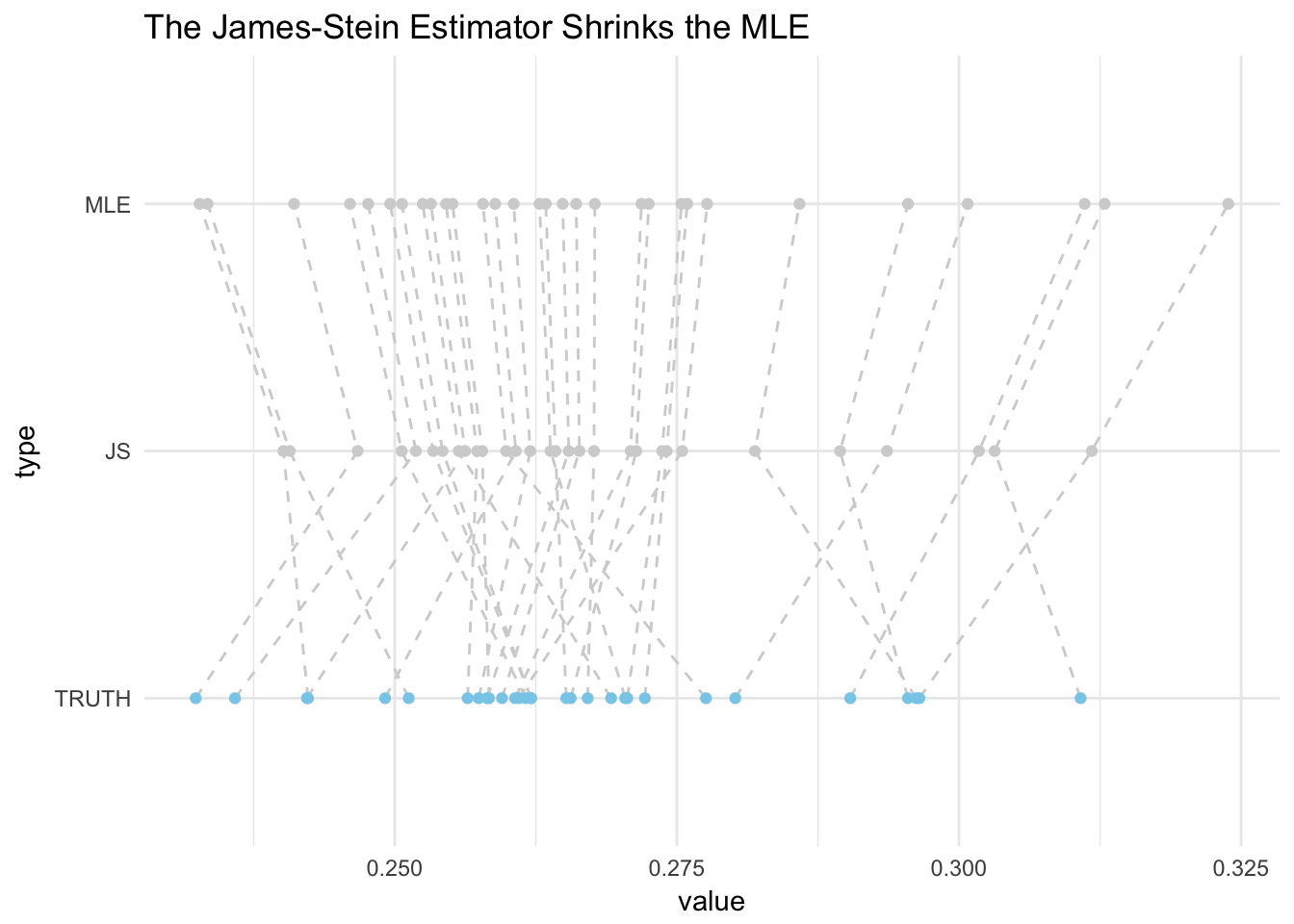
One thing to notice is that the James-Stein (JS) estimator shrinks estimates. Also, notice that some points are way off from the truth. Individually, the MLE seems to do better, but we are cuious to know if the JS is better over all. This can be tested by calculating the predictive squared error.

\[\sum_{i=1}^{30}(MLE_i-TRUTH_i)^2 = \]

errors <- df %>% 
  mutate(mle_pred_error_i = (MLE-TRUTH)^2,
         js_pred_error_i = (JS-TRUTH)^2) %>% 
  summarise(js_pred_error = sum(js_pred_error_i),
            mle_pred_error = sum(mle_pred_error_i))

Thus by example we prove the James-Stein Theorem

\[E\left[\left\lVert\hat{\mu}^{JS}-\mu\right\rVert^{2}\right]<E\left[\left\lVert\hat{\mu}^{MLE}-\mu\right\rVert^{2}\right]\] \[3.0\times10^{-3}<4.4\times10^{-3}\]

In this example the JS estimator beat the MLE by \(31\%\)! This is remarkable, but this was just one example. We ought to run our own simulation on the method, replicate the simulation on the method, then stretch the estimator to its limits with data tailored to be a challenge for it.

4.1.5 Simulation

This example is nice because I only have to worry about having more than 3 samples, as stated in James-Steins theroem and we need to draw from the following distribution.

\[x_i|\mu_i\sim N(\mu_i,1)\]

You will notice that in the baseball example we did above we used an approximation because we had binomial data. We will stick to this in out simulation, but you may want to run an analogous simulation using the parameters for the normal.

4.1.5.1 Binomial Approximation

\[x_i|p_in\sim N(p_in,p_in(1-p_i))\] \[p_i\sim Bin(n,p_i)\]

# build data with MLE estiamte
set.seed(42)
sim <- tibble(player = letters, 
              AB_total=300, 
              TRUTH = rbeta(100,300,n=26),
              hits_list = map(.f=rbinom,TRUTH,n=300,size=1)
)
bats_sim <- sim %>% 
  unnest(hits_list) %>% 
  group_by(player) %>% 
  summarise(Hits = sum(hits_list)) %>% 
  inner_join(sim, by = "player") %>% 
  mutate(MLE = Hits/AB_total) %>% 
  select(-hits_list)
bats_sim

# A tibble: 26 x 5
   player  Hits AB_total     TRUTH       MLE
    <chr> <int>    <dbl>     <dbl>     <dbl>
 1      a    65      300 0.2362555 0.2166667
 2      b    71      300 0.2590379 0.2366667
 3      c    82      300 0.2660844 0.2733333
 4      d    78      300 0.2600898 0.2600000
 5      e    62      300 0.2474129 0.2066667
 6      f    92      300 0.2929336 0.3066667
 7      g    80      300 0.2476917 0.2666667
 8      h    98      300 0.3126689 0.3266667
 9      i    82      300 0.2484695 0.2733333
10      j    90      300 0.2859101 0.3000000
# ... with 16 more rows

#calculate variables for JS estimator
p_=mean(bats_sim$MLE)
N = length(bats_sim$MLE)

# add JS to simulated baseball data 
bats_sim <- bats_sim %>% 
  mutate(sigma2 = (p_*(1-p_))/300,
         JS=p_+(1-((N-3)*sigma2/(sum((MLE-p_)^2))))*(MLE-p_)) %>% 
  select(-AB_total,-Hits,-sigma2)

# plot
bats_sim %>% 
  gather(type,value,2:4) %>% 
  mutate(is_truth=+(type=="TRUTH")) %>% 
  mutate(type = factor(type, levels = c("TRUTH","JS","MLE"))) %>%
  arrange(player, type) %>% 
  ggplot(aes(x=value,y=type))+
  geom_path(aes(group=player),lty=2,color="lightgrey")+
  scale_color_manual(values=c("lightgrey", "skyblue"))+ #truth==skyblue
  geom_point(aes(color=factor(is_truth)))+
  guides(color=FALSE)+ #remove legend
  labs(title="The James-Stein Estimator Shrinks the MLE")+
  theme_minimal()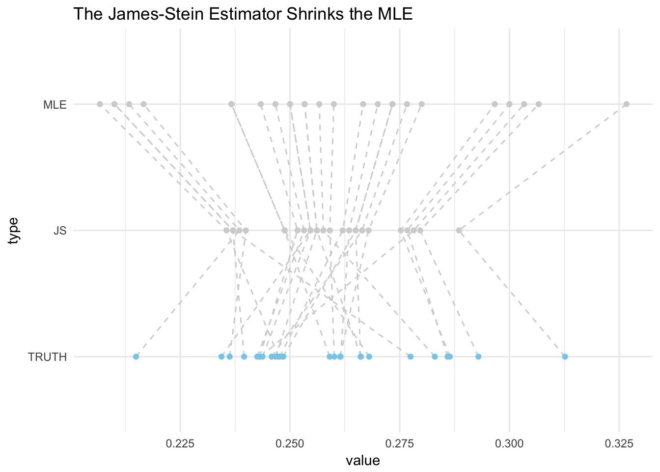

errors <- bats_sim %>% 
  mutate(mle_pred_error_i = (MLE-TRUTH)^2,
         js_pred_error_i = (JS-TRUTH)^2) %>% 
  summarise(js_pred_error = sum(js_pred_error_i),
            mle_pred_error = sum(mle_pred_error_i))
errors

# A tibble: 1 x 2
  js_pred_error mle_pred_error
          <dbl>          <dbl>
1    0.00752319     0.01685781

4.1.6 Excercise

Replicating Simulations: Using simulation test the James Stein estimator with the following sample sizes 2,3,10,30,100,1000.

This concludes our James-Stein estimator discussion, my hope is that the reader has gained some appreciation for the James-Stein estimator and learned a little about analysing properties of statistical methods.

4.1.7 Further Reading

Stein’s Paradox in Statistics, Bradley Efron
Why Isn’t Everyone A Bayesian, Bradley Efron
Computer Age Statistical Inference, Efron and Hastie
Simulation for Data Science with R, Matthias Templ