Part 3 Tidyverse Basics
library(tidyverse)The tidyverse is a
collection of R packages designed for data science. All packages share an underlying philosophy and common APIs.
Covering all of the tidyverse is beyond the scope of this book. What you will do is master the parts that are necessary for method testing. This includes parts of purrr, dplyr, tidyr, and tibble. All plots will be generated with ggplot2. I will show the code for plots in the book, but all code is available on my github.
3.1 Generating 5 Gaussian Random Variable
Lets start by generating 5 random variables from the normal distribution with mean 0 and standard deviation 1.
\[\begin{equation*} X\sim N(0,1) \end{equation*}\]rnorm(mean=0,sd=1,n=5)[1] -1.1045994 0.5390238 0.5802063 -0.6575028 1.5548955R provides many more distributions that we will use for data generation
| Distrubution | Notation | R |
|---|---|---|
| Uniform | \(U(a,b)\) | runif() |
| Normal | \(N(\mu,\sigma^2)\)* | rnorm() |
| Binomial | \(Bin(n,p)\) | rbinom() |
| Piosson | \(Pois(\lambda)\) | rpois() |
| Beta | \(Beta(\alpha,\beta)\) | rbeta() |
3.1.0.1 Exercise
Exercise use
?rpois()to learn about how this command works. Generate 3 random Poisson variables.
3.2 Using map() and %>%
We will want to make draws from the same distribution, but with different parameters. Lets generate three random normals with means 5, 15, -5.
mu <- list(5, 15, -5)
mu %>%
  map(rnorm, n = 5) %>%
  str()
List of 3
$ : num [1:5] 3.81 5.15 3.91 6.61 5.04
$ : num [1:5] 16.3 16 15.9 15.5 16
$ : num [1:5] -5.81 -4.72 -5.16 -3.06 -3.28The map() function is from the library purrr. This library provides many useful functions to abstract for loops. The abstraction lets us to a lot of work with relativly few lines of code. We can think of the map() as iterating rnorm for each of the mu supplied to it as follows:
| Notation | rnorm |
|---|---|
| \(X\sim N(5,1)\) | rnorm(mean=5,n=5) |
| \(X\sim N(15,1)\) | rnorm(mean=15,n=5) |
| \(X\sim N(-5,1)\) | rnorm(mean=-5,n=5) |
In the above lines of code we stored a list of means in the mu variable. We then passed mu into map() with the %>% – the “magrittr”, which is a pipe-like operator (x %>% f, rather than f(x)). The str() function is used to visualize data in a compact way.
3.2.0.1 Exercise
Generate 3 Poisson random variables with parameters equal to 0,1,2 each with length 10.
3.3 Using pmap() and tribble
We may want to specify two parameters in a distribution.
params <- tribble(
 ~n, ~mean, ~sd,
 10,    0,    1,
 20,    5,    1,
 30,    10,   2
)
params %>%
  pmap(rnorm) %>%
  str()
List of 3
$ : num [1:10] 0.358 0.302 -0.394 0.788 0.671 ...
$ : num [1:20] 5.95 4.3 3.92 4.95 5.58 ...
$ : num [1:30] 11.25 4.32 11.96 9.76 10.19 ...The tribble function is a way to create a tibble by row. You can think of it is a mini csv. The column headers begin with ~ and values are separated by a comma.
The pmap() function takes any number of parameters into the function. This is powerful because we can specify the different parameters and lengths for sampling from.
3.3.0.1 Exercise
Usepmap()to generate three Binomial random variables \[\begin{equation*} X\sim Bin(n,p) \end{equation*}\]. If you need help with the parameterization use
?rbinomfor help.
3.3.0.2 Exercise
What happens when you run the following and why?
params <- tribble(
 ~n, ~mu, ~sigma,
 10,    0,    1,
 20,    5,    1,
 30,    10,   2
)
params %>%
  pmap(rnorm) %>%
  str()
3.4 Using invoke_map() and mutate()
The pmap() example was still simplistic. We could have added complexity by adding more than one distribution, each with different parameterizations.
library(tidyverse)
f <- c("runif", "rnorm", "rpois")
param <- list(
  list(min = -1, max = 1),
  list(sd = 5),
  list(lambda = 10)
)
invoke_map(f, param, n = 10) %>% str()
List of 3
$ : num [1:10] -0.366 -0.768 -0.628 0.459 -0.176 ...
$ : num [1:10] 1.17 3.68 5.46 -3.23 3.33 ...
$ : int [1:10] 6 13 13 6 9 7 8 9 10 10A table of invoke_map would look like the following
f |
param |
invoke_map(f,param,n=10) |
|---|---|---|
runif() |
min= -1,max= 1 |
runif(min=-1,max=1,n=10) |
rnorm() |
sd=5 |
rnorm(mean=0,sd=5,n=10) |
rpois() |
lambda=10 |
rpois(lambda=10,n=10) |
We could also use a tribble instead of a list. Notice that the code below is the same as above except that the data is stored in a tribble and the length of the vectors are different.
sim <- tribble(
  ~f,      ~params,
  "runif", list(min = -1, max = 1,n=10),
  "rnorm", list(sd = 5, n=15),
  "rpois", list(lambda = 10,n=30)
)
sim %>%
  mutate(sim = invoke_map(f, params))
# A tibble: 3 x 3
f params sim
<chr> <list> <list>
1 runif <list [3]> <dbl [10]>
2 rnorm <list [2]> <dbl [15]>
3 rpois <list [2]> <int [30]>In the above command we generate values from a number of distributions that have different parameterizations, with different lengths. We also end up with columns that have lists in each cell. This is called a list column. List columns are mentioned more in the next section.
3.4.0.1 Exercise
Create a tribble with the binomial, normal, and beta distribution. Select a different number of parameters for each distibution. Then use invoke_map to make a column holding the sample as was done in the above code.
3.5 crossing() and list columns
Before introducing the crossing() function lets set up a simple ,albiet cliche, coin flipping experiment. We flip a coin 10 times and observe the average. Here our random variable is distributed as
\[\begin{equation*}
X_{\text{One Experiment}}\sim Bin(10,0.5)
\end{equation*}\]
, where
\[\begin{equation*}
\bf{x}\in \mathcal{R}^{10}.
\end{equation*}\]
The blow code is just one hypothetical experiment. If you run the code many times you will likely get different answers.
#1. One Experiment
n_tosses=10
one_exp <- rbinom(p=0.5,size=1,n_tosses)
mean(one_exp)
We know that the probability of getting a “heads” is 0.5. We normally don’t know exact probabilities, but in this simple example we do. We can test this to see if 0.5 is the expected value from this experiment by replicating it.
The following code does the same thing as the code above it, but we set it up slightly different to it will be easy for us to add replications.
#2. Setup For Replication
sim <- tribble(
  ~f,      ~params,
  "rbinom", list(size = 1, prob = 0.5)
)
sim %>%
  mutate(sim = invoke_map(f, params, n = 10)) %>%
  unnest(sim) %>%
  summarise(mean_sim = mean(sim))
Now lets add some replications.
#3. Replicate 1e4 Times
sim <- tribble(
  ~f,      ~params,
  "rbinom", list(size = 1, prob = 0.5)
)
rep_sim <- sim %>%
  crossing(rep = 1:1e5) %>%
  mutate(sim = invoke_map(f, params, n = 10)) %>%
  unnest(sim) %>%
  group_by(rep) %>%
  summarise(mean_sim = mean(sim))
head(rep_sim)
# A tibble: 6 x 2
rep mean_sim
<int> <dbl>
1 1 0.3
2 2 0.6
3 3 0.7
4 4 0.3
5 5 0.5
6 6 0.6The above code was a handful. We can break it up into peices to see what is happening.
# Chunk 1
rep_sim <- sim %>%
  crossing(rep = 1:1e5) %>%
  mutate(sim = invoke_map(f, params, n = 10))
head(rep_sim)
# A tibble: 6 x 4
f params rep sim
<chr> <list> <int> <list>
1 rbinom <list [2]> 1 <int [10]>
2 rbinom <list [2]> 2 <int [10]>
3 rbinom <list [2]> 3 <int [10]>
4 rbinom <list [2]> 4 <int [10]>
5 rbinom <list [2]> 5 <int [10]>
6 rbinom <list [2]> 6 <int [10]>If we stop immediatly after the mutate you will see that rep_sim — up to this point — is a tidy data frame. The sim column is a little different from a single value, it is a list. sim is what we is called a list column. Values in list columns are nested. If we want to summarize each of the results from the 10,000 experiments we need to unnest them with the unnest() command.
In the below chunk we unnest by sim. Then we group by the replications, this is the 10,000 runs we did. In many cases you will use group_by to precede summarise. By doing a group_by before summarize we are capturing the mean for each of the 10,000 replications.
rep_sim <- sim %>%
  crossing(rep = 1:1e5) %>%
  mutate(sim = invoke_map(f, params, n = 10)) %>%
  unnest(sim) %>%
  group_by(rep) %>%
  summarise(mean_sim = mean(sim))
head(rep_sim)
# A tibble: 6 x 2
rep mean_sim
<int> <dbl>
1 1 0.4
2 2 0.3
3 3 0.3
4 4 0.4
5 5 0.6
6 6 0.4We can now visualize the means of all of our replication to see if 0.5 is a good expected value.
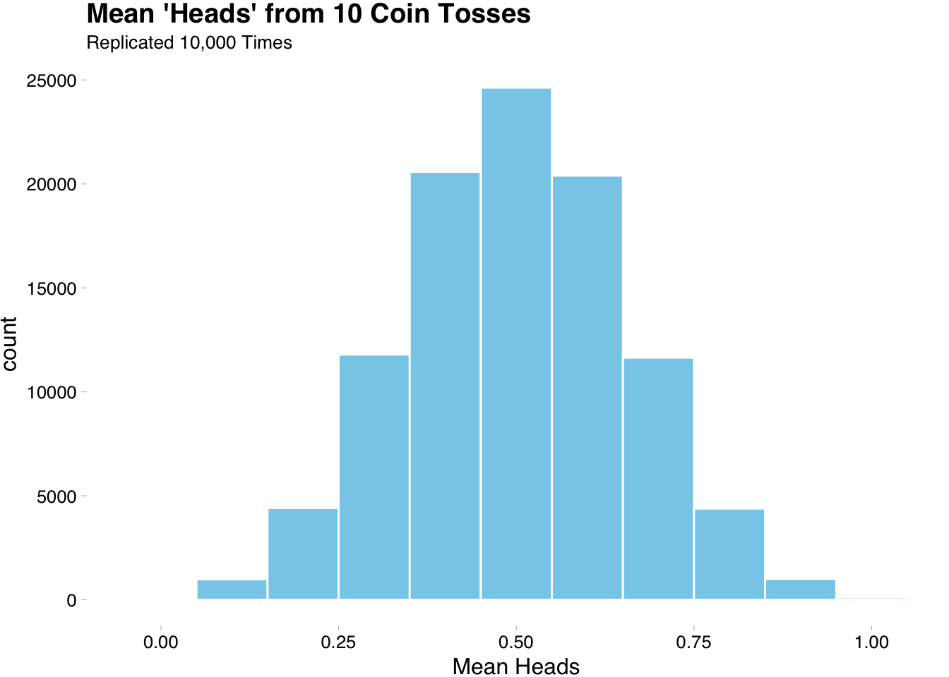
The above plot is nice, but it does not get at the heart of what we want to know. If we want to know that 0.5 is a good expected value we need to see what happens as the number of trials approach a large number. We will get more tidyverse practice by exploring this more in the next section.
3.5.0.1 Exercise
Repeat the above code, but use a biased coin. Chose the bias by changing the
probargument in therbinomfunction.
3.6 Law of Large Numbers — Tidyverse Practice
If 0.5 represents a good “long-run” estimate for our coin flipping then the outcome variable of interest should represent the error or difference between what a trial gets and what we know is the truth (0.5). Lets create data that will allows us to visualize what happens to the error as the number or trials gets big. To be clear we are no longer interested in doing replications with the same number of trials. We want to replicate with changing values for the number of tosses and capture the distance from 0.5.
set.seed(42)
params <- tribble(
  ~size, ~prob,
    1,     0.5
)
p <- params %>%
  crossing(n=1:1e4) %>%
  pmap(rbinom) %>%
  enframe(name="num_toss",value="observation")
You can see that observation is a list that increases in size. We will now group_by num_toss and summarize the distance from 0.5.
p <- params %>%
  crossing(n=1:1e4) %>%
  pmap(rbinom) %>%
  enframe(name="num_toss",value="observation") %>%
  unnest(observation) %>%
  group_by(num_toss) %>%
  summarise(vale = mean(observation))
Of course, we can still do better. This was just one go at changing the number of tosses. Maybe we got lucky. Lets run multiple replications of the above experiment.
sim <- tribble(
 ~n_tosses, ~f,       ~params,
  10, "rbinom", list(size=1,prob=0.5,n=15),
  30, "rbinom", list(size=1,prob=0.5,n=30),
  100, "rbinom", list(size=1,prob=0.5,n=100),
  1000, "rbinom", list(size=1,prob=0.5,n=1000),
  10000, "rbinom", list(size=1,prob=0.5,n=1e4)
)
sim_rep <- sim %>%
  crossing(replication=1:50) %>%
  mutate(sims = invoke_map(f, params)) %>%
  unnest(sims) %>%
  group_by(replication,n_tosses) %>%
  summarise(avg = mean(sims))
sim_rep %>%
ggplot(aes(x=factor(n_tosses),y=avg))+
ggbeeswarm::geom_quasirandom(color="lightgrey")+
scale_y_continuous(limits = c(0,1))+
geom_hline(yintercept = 0.5,
color = "skyblue",lty=1,size=1,alpha=3/4)+
ggthemes::theme_pander()+
labs(title="50 Replicates Of Mean 'Heads' As Number Of Tosses Increase",
y="mean",
x="Number Of Tosses")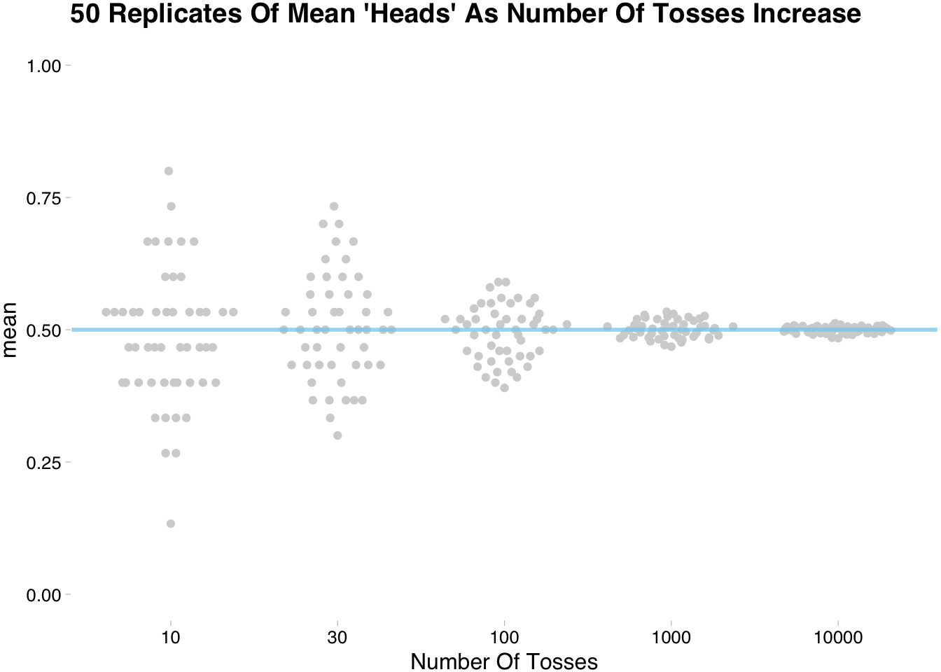
The above plot shows that the more tosses we do the closer we get to the expected value. This somewhat trivial for the coin flipping example, but when testing unfamiliar methods/estimates the technique of simulating replications comes in handy. If this is unfamiliar go ahead and repeat the above code and play with different distributions.