Chapter 3 Hieracrchial Clustering

Hierarchical Clustering seeks to build clusters by either breaking clusters apart or clumping them together based on the distance between two observations. An overview on how this works is you begin by either putting subjects into one cluster or into their own separate cluster. You then find the distance between the two subjects and then based on the criteria of your choosing you would clump or merge two subjects into one cluster. You would then repeat this process of finding the distance between the subjects and clusters once you have formed then creating new clusters.

3.1 Distance Component

We mentioned how you first want to find the distance between all observations to begin the process of hierarchical clustering. This is important because this is how measure of how similar our observations are. The distance you want to find is known as Euclidean Distance. We touched on matrix algebra early and this is important because we will be using the matrix form of the euclidean distance. The euclidean distance between two vectors, or matrices, takes on the following form;

\[ d(x,y) = \sqrt{\sum_{i=1}^p (x_i - y_i)^2} = \sqrt{(x-y)^{'}(x-y)} \]

where d denotes the distance between the two vectors and p is the number of variables.

3.2 Measure of Distance

Once we have found the distance between our observations we must then decide how we to create our clusters. This part is also subjective and there are many approaches to which it can be done. One that we would like to focus on is what is called single linkage. How single linkage works is once you find the distances between your observations the distance between two clusters is defined as the minimum distance. Once you find the minimum distance between your clusters you then group together the clusters or observations.

3.3 Spotify Example

We feel the greatest way to see how this method can be applied is to run through a real life example.

The dataset we will be exploring is on songs of spotify. The dataset contains songs characteristics such as loudness, dance ability, key, etc, and can be found here.

Since the data set is very large and the computations extensive, we will run through a random sample of 10 observations which is shown in Table 3.1 to allows us to show how this process works.

Table 3.1: Spotify Songs of 10 observations

Genre	danceability	energy	key	loudness	mode	speechiness	acousticness	instrumentalness	liveness	valence	tempo
RnB	0.767	0.611	5	-5.173	0	0.0983	0.15700	0.01160	0.0836	0.110	188.068
trance	0.628	0.873	0	-6.680	1	0.0634	0.00202	0.57000	0.5390	0.128	130.005
psytrance	0.570	0.868	1	-5.760	0	0.0573	0.00466	0.49200	0.3350	0.159	139.974
Underground Rap	0.709	0.633	2	-7.612	1	0.3000	0.01030	0.00000	0.0710	0.575	154.124
Dark Trap	0.525	0.651	8	-9.845	0	0.0551	0.14400	0.00181	0.1070	0.323	163.909
Hiphop	0.544	0.812	1	-6.431	1	0.3930	0.01850	0.00000	0.4810	0.678	183.529
techhouse	0.698	0.965	10	-5.616	0	0.1120	0.01120	0.01470	0.1110	0.499	123.994
hardstyle	0.480	0.959	2	-5.165	0	0.1980	0.00179	0.03230	0.5330	0.239	149.804
Rap	0.742	0.711	10	-4.658	1	0.2370	0.06140	0.00623	0.1240	0.294	175.903
techhouse	0.803	0.574	6	-11.681	1	0.0808	0.00205	0.93300	0.1120	0.333	126.018

For this example, lets say Spotify came to us, I know how awesome would that be, and wanted us to group together similar genres for a local tour they are putting together. They want to group similar genres for certain days that best fit each other. Running through these 10 observations will give us an understanding of how this process might be down.

Step 1

The way we are going to approach this problem is by first considering that every observation is its own cluster. Now we want to find the euclidean distance between our observations, to do so we would treat each row as a vector. Therefore, row 1 would like the following in vector form;

\(y_1^{'}\) = (0.767 0.611 5 -5.173 0 0.0983 0.15700 0.01160 0.0836 0.110 188.068)

similarly for row 2;

\(y_2^{'}\) = (0.628 0.873 0 -6.680 1 0.0634 0.00202 0.57000 0.5390 0.128 130.005).

Then we would compute the distance from the formula we mentioned earlier in this section.

\[ d(y_1,y_2) = \sqrt{(.767 - .628)^2 + (.611 - .873)^2 + ...+(188.068 - 130.005)^2} \approx 5 \]

With some rounding being done we would then say that the distance between observation 1 and observation 2 is 5. You would then proceed in this fashion between all observations. Using software can make this task more efficient because you can see how tedious this can be once you go past three variables. Once you compute all these distance you can store them in whats called a distance matrix.

Table 3.2: Distance Matrix of 10 Observations

1	2	3	4	5	6	7	8	9	10
0	5	4	4	6	4	5	3	5	7
5	0	2	2	9	1	10	3	10	8
4	2	0	2	8	1	9	1	9	8
4	2	2	0	6	2	8	3	9	6
6	9	8	6	0	8	5	8	6	3
4	1	1	2	8	0	9	2	9	7
5	10	9	8	5	9	0	8	1	7
3	3	1	3	8	2	8	0	8	8
5	10	9	9	6	9	1	8	0	8
7	8	8	6	3	7	7	8	8	0

Step 2

Now that you have created your distance matrix, you will know begin the clustering process. First, you find the overall minimum distance between two different observations. In this example, we can see that there are multiple observations that have a distance of 1 from each other, in this case we would initially cluster these observations together. Now you repeat the step we did above finding the distance between each observation and the distance between the observations and the clusters. This is where single linkage comes into play, once you have created your initial clusters, the distance between an observation and a cluster is the minimum distance between the observation and one of the observations in the cluster.

For our example, lets say we initially clustered observation 2 and observation 6 together because they have a distance of 1 which is the minimum distance overall. When we go to create our new distance matrix if we wanted to find the distance between observation 1 and this cluster of 2 and 6, we would find the distance between observation 1 and observation 2. Then we would find the distance between observation 1 and observation 6. We use the original distances we calculated up above, so the distance between observation 1 and 2 have a measure of 5. The distance between observation 1 and 6 have a measure of 4. The single linkage method would use the distance of 4 because that is the minimum distance between observation 1 and the cluster of 2 and 6 so you would update that numeric value into the distance matrix. You would then proceed to do this for every observation and cluster, finding the overall minimum distance and either creating new cluster of joining observations into the clusters. You repeat this process until there is only 1 cluster left which is all observations joined together.

Dendrogram

Once you finished your clustering there are nice visualizations you can create, one popular one is called a dendrogram. A dendogram is essentially a easy way to show where your clusters form and what observations are joined together.

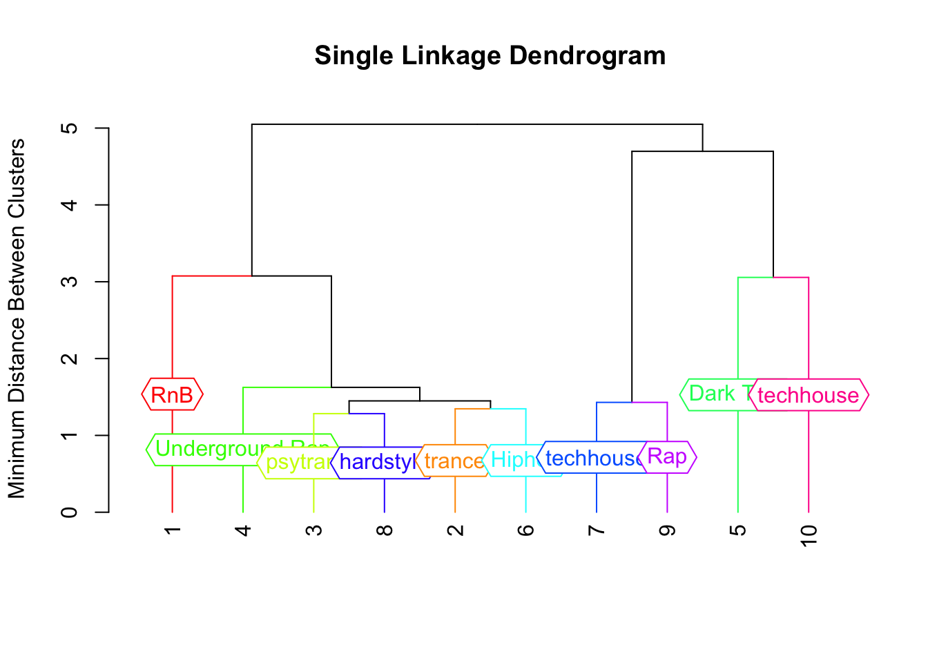
Figure 3.1: Spotify Genre Grouping

Summary

Figure 3.1 gives a great visualization of how this process works. All observations are initially in their own cluster and you can see when each cluster is formed. So for our example lets say Spotify is having their tour on a Friday and Saturday so they want two clusters from this data set. Based on this sample we worked with we would tell them that RnB, Underground Rap, Psytrance, Hard style, Trance and Hip hop are similar to each other so they should plan on having these genres on one day. Tech house, Rap, and Dark Trap are similar to each other based on our analysis so those genres should be on a separate day. Since we only worked with 10 observations this is not a great representation of the actual clusters but this is the idea that cluster analysis strives for.