Chapter 4 Online Classes

4.1 Machine Learning

• Currently taking two courses on machine learning
• Practical Machine Learning with R on Coursera
• Applied Machine Learning via FAES

4.1.1 Practical Machine Learning

4.1.1.1 Why Preprocess?

• Features can be very skewed

• preProcess function in the caret package allows for standardization/normalization of data

  • Can use a preProcess object to adjust other subsets (eg. test set)
  • preProcess argument exists within train function

• BoxCox transforms take continuous data, and attempts to make them look like normal data

• Can also impute data

  • Various methods such as knnImpute

• Training and test set must be processed in the same way

• Test transformations will likely be imperfect

  • Especially if the sets are collected at different times

• Be careful when transforming factor variables

4.1.1.2 Covariate Creation

Two levels of covariate creation

1. From raw data to covariate

• Converting text into token counts

2. Transforming tidy covariates

• Functional transformations (log, etc)

• Level 1

  • Depends on application
  • summarization vs information loss
  • when in doubt, stay on the side of more features
  • can be automated, but use caution

• Level 2

  • More necessary for some methods (regression, svms)
  • Only on the training set
  • Discovery through EDA
  • New covariates should be added to data frames (don’t removed original)

• use nearZeroVar function in caret to remove unimportant features

• library(splines) to create a bs basis

  • creation of polynomial variables to then fit
  • fitting curves w/splines

4.1.1.3 Preprocessing with Principal Components Analysis

• Use with many correlated predictors
• Weighted combination of predictors
• Reduced predictors/noise
• Find a new set of variables that are uncorrelated and explain as much variance as possible
• Find the best matrix with fewer variables (lower rank) that explains the original data
• Related solutions - SVD and PCA
• prcomp in R
• Can preprocess with PCA in caret
• Have to use same PCA in test set
• Make sure to transform first

4.1.1.4 Quiz 2

library(AppliedPredictiveModeling)
library(caret)
data(AlzheimerDisease)

4.1.1.4.1 Question 1

adData = data.frame(diagnosis,predictors)
trainIndex = createDataPartition(diagnosis, p = 0.50,list=FALSE)
training = adData[trainIndex,]
testing = adData[-trainIndex,]

4.1.1.4.2 Question 2

library(Hmisc)
library(tidyverse)
data(concrete)
set.seed(1000)
inTrain = createDataPartition(mixtures$CompressiveStrength, p = 3/4)[[1]]
training = mixtures[ inTrain,]
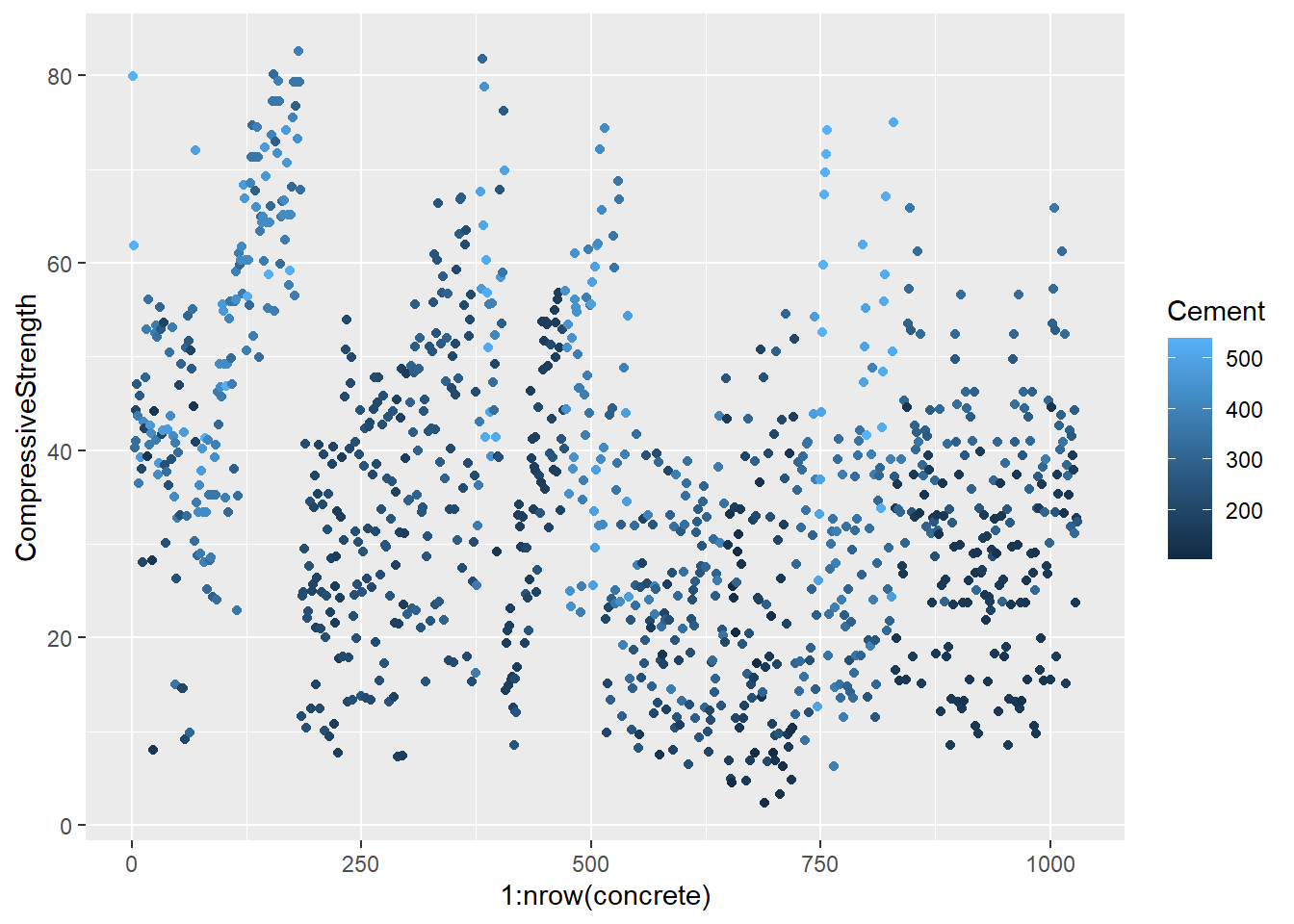
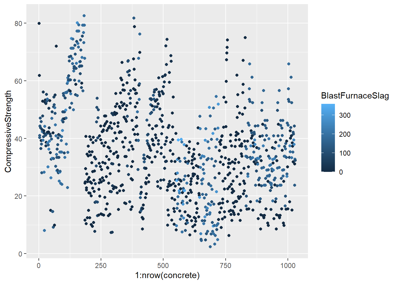
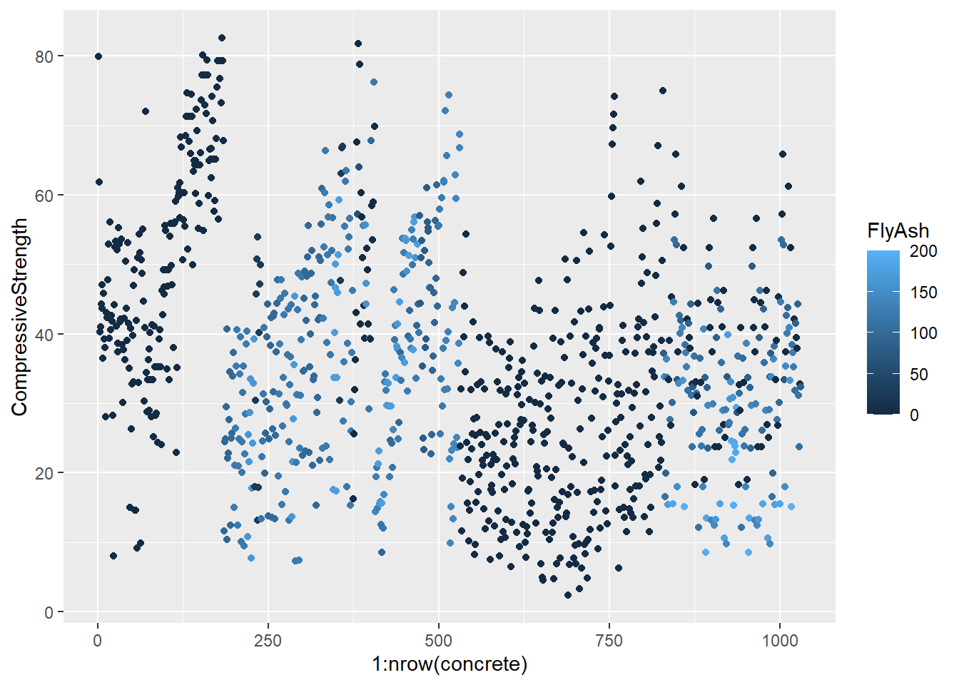
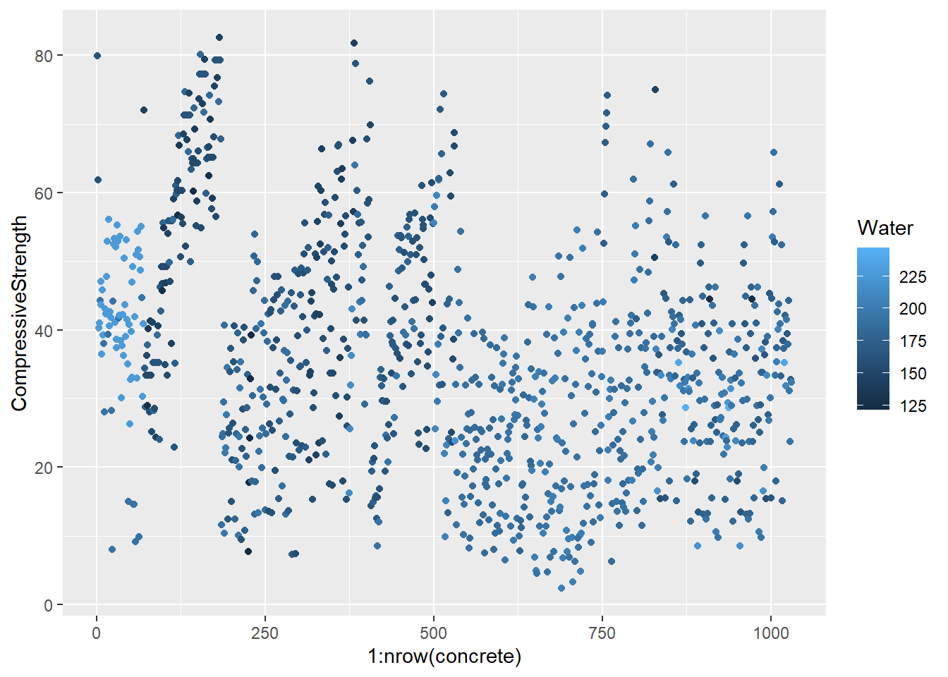
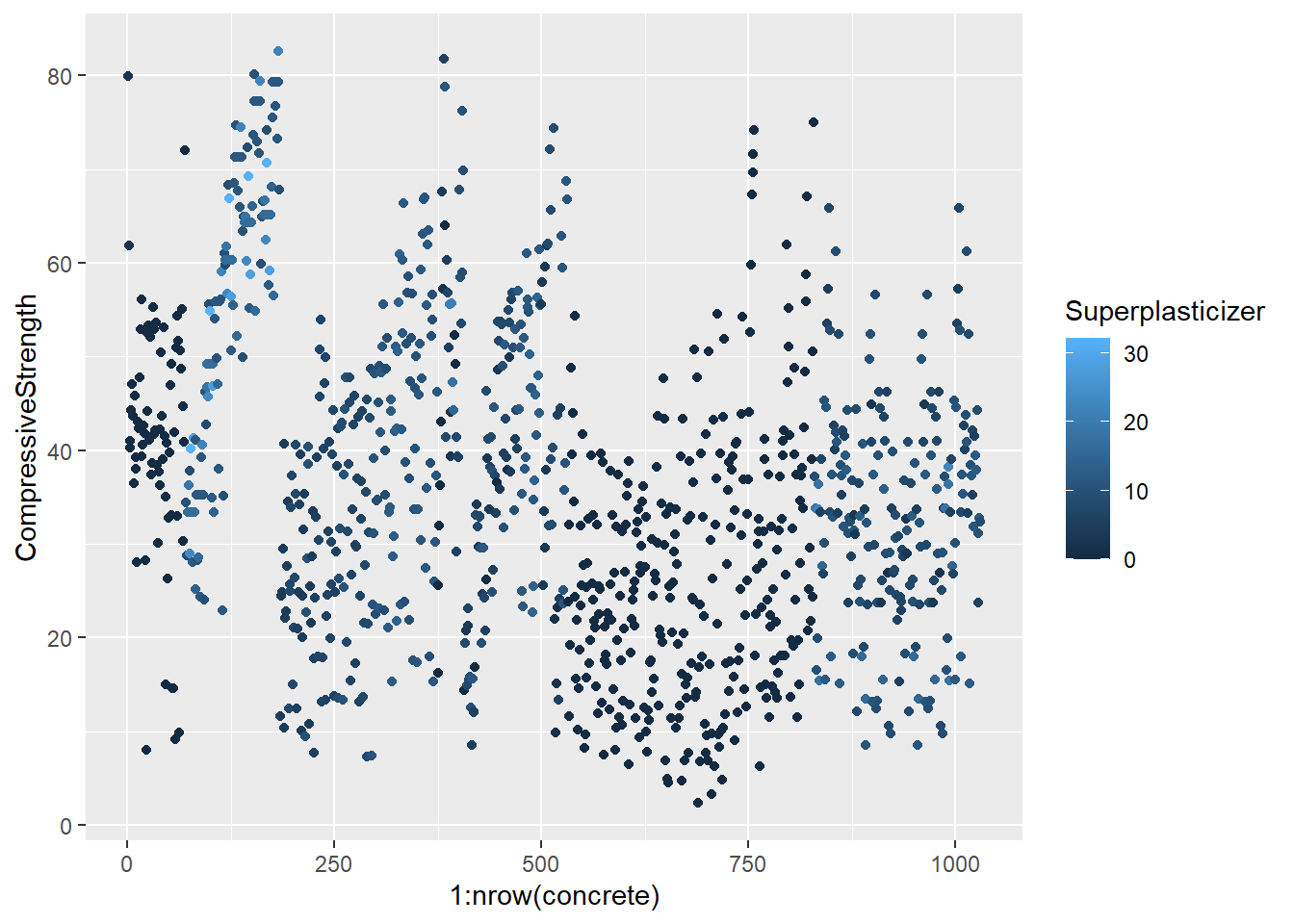
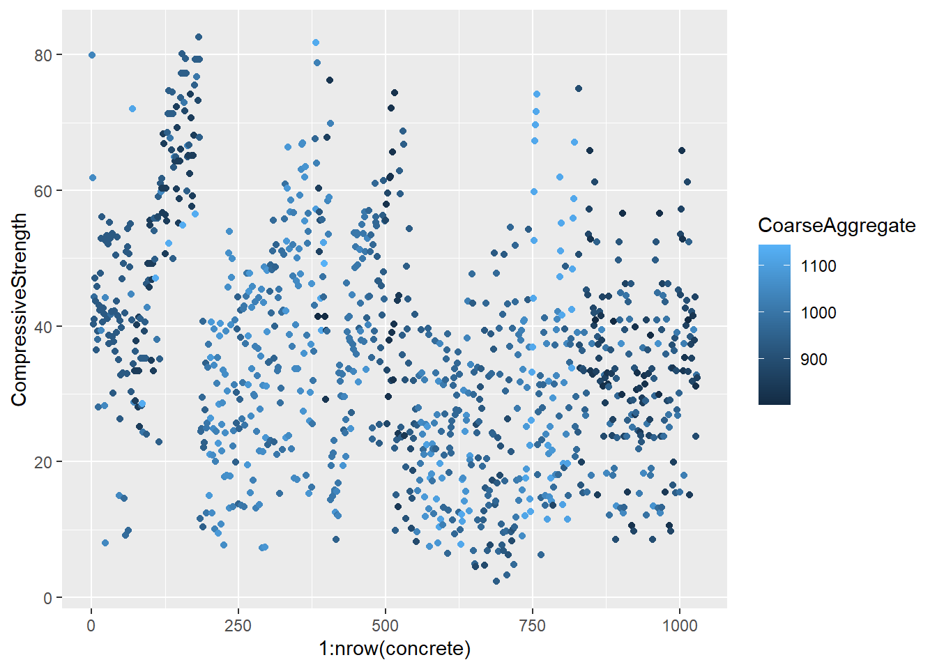
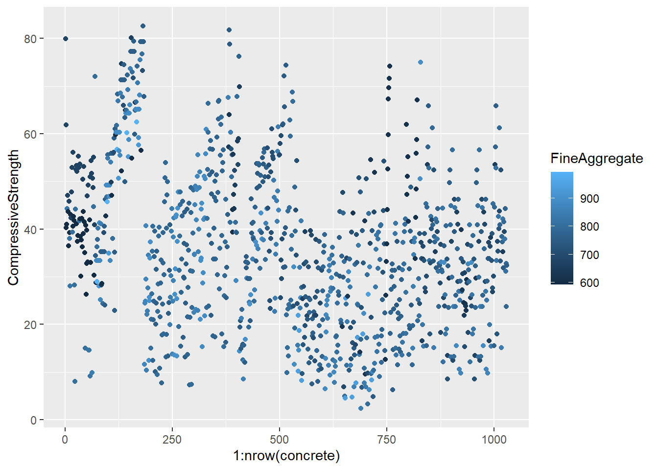
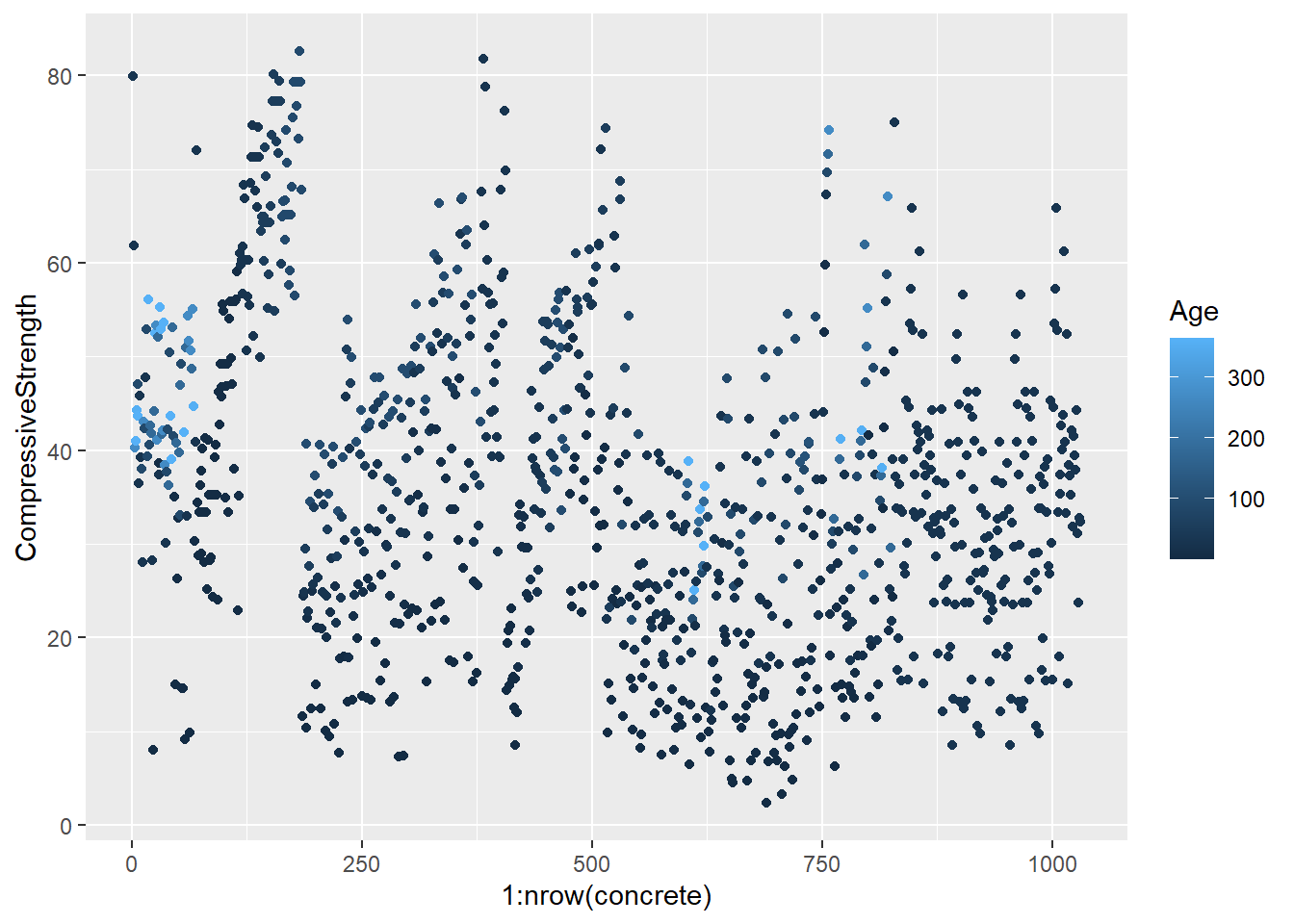
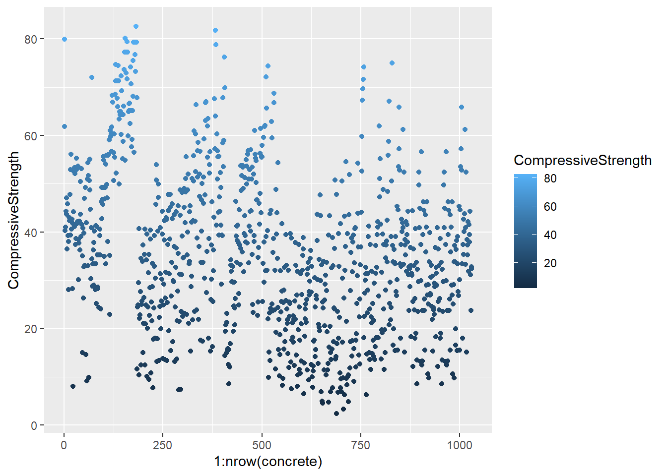
testing = mixtures[-inTrain,]

Make a plot of the outcome (CompressiveStrength) versus the index of the samples. Color by each of the variables in the data set (you may find the cut2() function in the Hmisc package useful for turning continuous covariates into factors). What do you notice in these plots?

base_plot <- ggplot(concrete, aes(1:nrow(concrete), CompressiveStrength)) +
  geom_point()

for (x in names(concrete)) {
  print(
    base_plot + 
    aes_string(col = x)
  )
}

4.1.1.4.3 Question 3

data(concrete)
set.seed(1000)
inTrain = createDataPartition(mixtures$CompressiveStrength, p = 3/4)[[1]]
training = mixtures[ inTrain,]
testing = mixtures[-inTrain,]

Make a histogram and confirm the SuperPlasticizer variable is skewed. Normally you might use the log transform to try to make the data more symmetric. Why would that be a poor choice for this variable?

ggplot(training, aes(Superplasticizer)) +
  geom_histogram()

## `stat_bin()` using `bins = 30`. Pick better value with `binwidth`.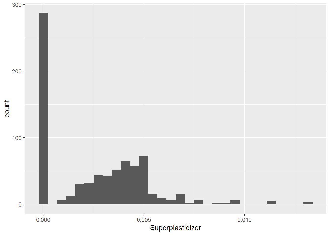

ggplot(training, aes(log(Superplasticizer))) +
  geom_histogram()

## `stat_bin()` using `bins = 30`. Pick better value with `binwidth`.

## Warning: Removed 287 rows containing non-finite values (stat_bin).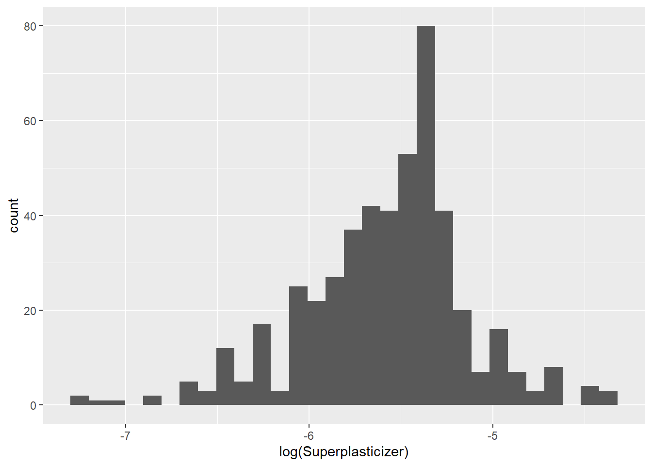

4.1.1.4.4 Problem 4

set.seed(3433)
data(AlzheimerDisease)
adData = data.frame(diagnosis,predictors)
inTrain = createDataPartition(adData$diagnosis, p = 3/4)[[1]]
training = adData[ inTrain,]
testing = adData[-inTrain,]

Find all the predictor variables in the training set that begin with IL.

names(
  training %>%
    select(
      starts_with("IL")
    )
)

##  [1] "IL_11"         "IL_13"         "IL_16"         "IL_17E"       
##  [5] "IL_1alpha"     "IL_3"          "IL_4"          "IL_5"         
##  [9] "IL_6"          "IL_6_Receptor" "IL_7"          "IL_8"

Perform principal components on these variables with the preProcess() function from the caret package. Calculate the number of principal components needed to capture 80% of the variance. How many are there?

il_training <- training %>%
  select(
    starts_with("IL")
  )

preProcess(il_training, method = "pca", thresh = 0.8)

## Created from 251 samples and 12 variables
## 
## Pre-processing:
##   - centered (12)
##   - ignored (0)
##   - principal component signal extraction (12)
##   - scaled (12)
## 
## PCA needed 7 components to capture 80 percent of the variance