2 GEE Basics
2.1 Signing up
- Go to: code.earthengine.google.com
- Earth Engine will now request access to your Google account, click ‘allow’.
- Click the link to go to the registration page, fill out the application and submit.
- After you receive your ‘Welcome to Google Earth Engine!’ email, you will be able to login using your Google account on: code.earthengine.google.com
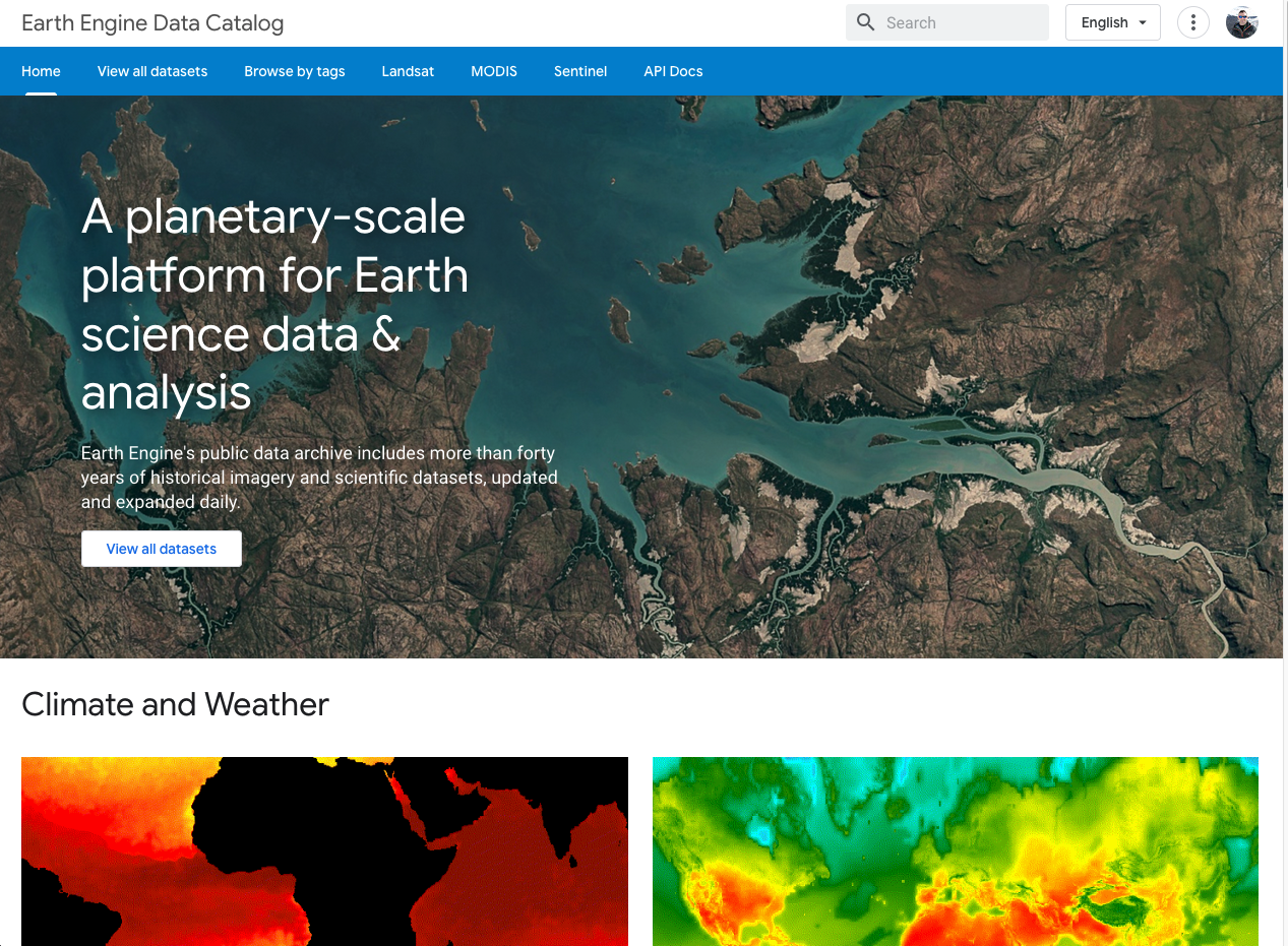
2.2 The code editor
Here is where all the work is done. In this API you can enter, edit, and run javascript code
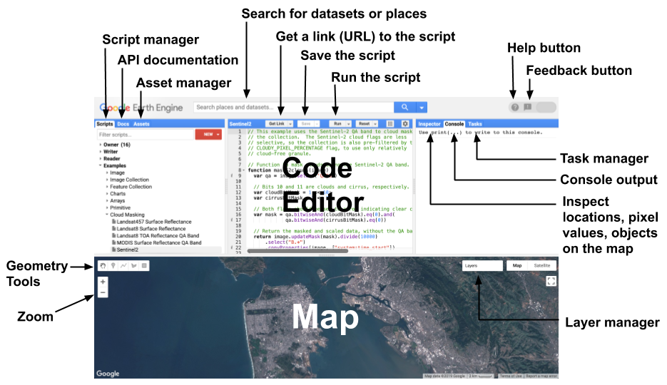
Figure 2.1: Earth Engine Code Editor, https://developers.google.com/earth-engine/guides/playground
Try entering some code and running it.
print('hello bioacoustics class');

// Variables
var city = 'Edmonton';
var country = 'Alberta';
print(city, country);

var population = 8400000;
print(population);

// List
var coolBirds = ['canada warbler', 'ovenbird', 'yellow rail', 'black-capped Chickadee'];
print(coolBirds);

// Dictionary
var cityData = {
  'city': city,
  'population': population,
  'elevation': 645
};
print(cityData);

// Function
var greet = function(name) {
    return 'Hello ' + name;
};
print(greet('bioacoustics class'));

// This is a comment
2.3 Adding data
Javascript syntax for different types of spatial data:
- Images (raster) objects:
- ee.Image – a single raster
- ee.ImageCollection – a set of images/rasters
- Feature (points, polygon,lines) objects:
- ee.Feature (composed of geometry)
- ee.FeatureCollection (multiple features)
Image collections
To load a collection explore available image collections in GEE’s data catalog
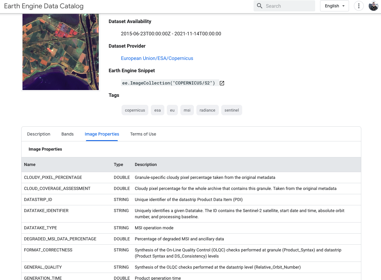
Here you can get information on each data set and the code needed to load a collection into the code editor. Visit the Sentinel-2, Level 1C page Sentinal-2, Level 1C page

Click on the tabs to read about sentinel, the available spectral bands, image properties, etc. There are two options for loading sentinel. You can copy the Earth Engine Snippet in the collection description. This will direct your code to load the collection.
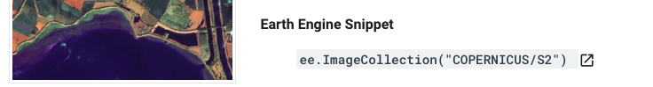
For more options, scroll down to the code under the Explore in Earth Engine heading. This code is a good starting point for loading, filtering, and visualizing the data set. Copy and paste the code into your editor. You can follow this process for all data collections in the GEE catalog.
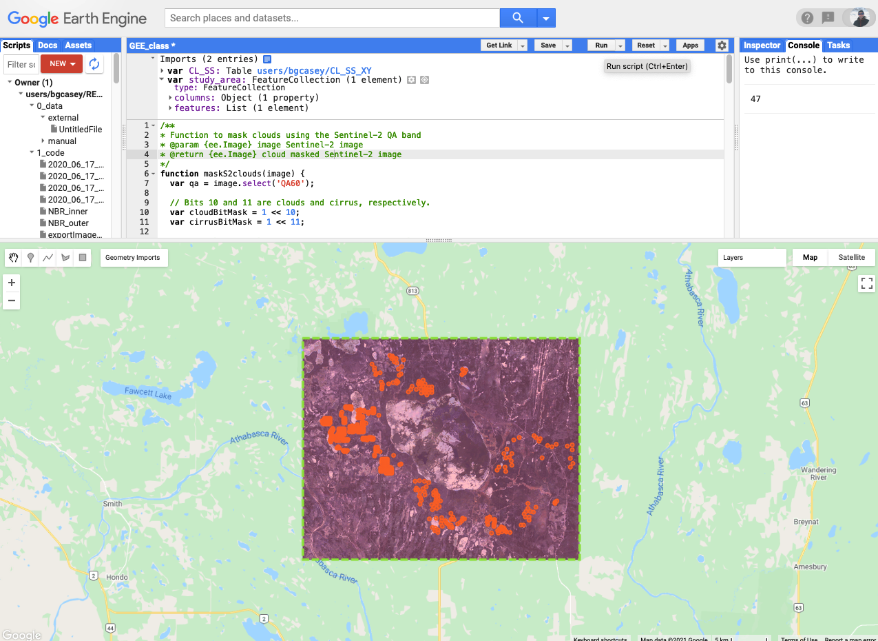
/**
 * Function to mask clouds using the Sentinel-2 QA band
 * @param {ee.Image} image Sentinel-2 image
 * @return {ee.Image} cloud masked Sentinel-2 image
 */
function maskS2clouds(image) {
  var qa = image.select('QA60');

  // Bits 10 and 11 are clouds and cirrus, respectively.
  var cloudBitMask = 1 << 10;
  var cirrusBitMask = 1 << 11;

  // Both flags should be set to zero, indicating clear conditions.
  var mask = qa.bitwiseAnd(cloudBitMask).eq(0)
      .and(qa.bitwiseAnd(cirrusBitMask).eq(0));

  return image.updateMask(mask).divide(10000);
}

// Map the function over one year of data and take the median.
// Load Sentinel-2 TOA reflectance data.
var dataset = ee.ImageCollection('COPERNICUS/S2')
                  .filterDate('2018-01-01', '2018-06-30')
                  // Pre-filter to get less cloudy granules.
                  .filter(ee.Filter.lt('CLOUDY_PIXEL_PERCENTAGE', 20))
                  .map(maskS2clouds);

var rgbVis = {
  min: 0.0,
  max: 0.3,
  bands: ['B4', 'B3', 'B2'],
};

Map.setCenter(-9.1695, 38.6917, 12);
Map.addLayer(dataset.median(), rgbVis, 'RGB');
In the code snippet, scroll to the function Map.setCenter(). The function sets the center point and zoom for the image. Change the coordinates listed here to the coordinates for Edmonton. The third number sets the zoom level. You can also edit the layer name as it appears on the map by changing ‘Map.addLayer(data set.median(), rgbVis, ’RGB’)’ to ‘Map.addLayer(data set.median(), rgbVis, ’Sentinel RGB’)’ Click run and wait for sentinel to load in the map viewer.
Feature collection
Where as image collections are collections rasters, feature collections are collections of geometric features (analogous to polygons, points, and lines in ArcGIS). You can import features using the method described above (searching the GEE catalog) or you can add your own features.
Import point features from a CSV.
Next we will upload our own features: point count station locations around calling Lake.
Download the data:
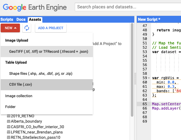
Download CL_SS_XY.csvWe will start by adding points from the calling lake csv. Click on the asset tab>new>CSV file, .
Select the file to upload, and scroll down to specify spatial properties. You can specify the XY fields and the CRS. CRS should be EPSG:4326
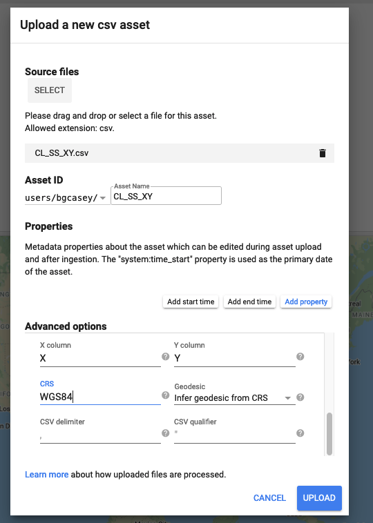
View upload progress by clicking on the task tab. Sometimes you need to refresh the asset list to see your newly imported asset. Once imported, click on the asset name. A pop-up window will appear. Here you can view and edit the asset’s description and properties. Click the import button.

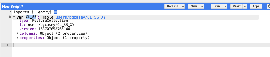
You will see a new code snippet at the top of the code editor. Click on var “table” to change the feature name from “table” to “CL_SS”
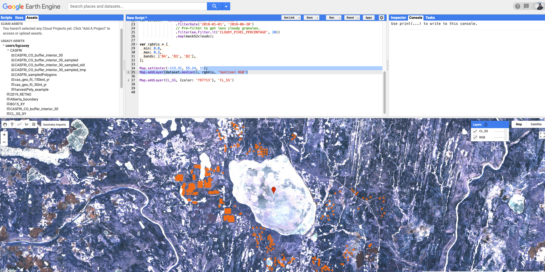
To view the points in your map window enter the following. Also change Map.setCenter values to -113.31, 55.24, 12 to zoom on Calling Lake.
Map.addLayer(CL_SS, {color: 'f87713'}, 'CL_SS')

//center map on Calling lake
Map.setCenter(-113.31, 55.24, 11)
Click run. Once the layers load you can click on the Layers button to toggle layers.
Create a feature using the map viewer
You can also create geometric features using drawing tools in the map viewer. Click on the rectangle drawing tool and use it to define a study area around your Calling Lake points. The new geometry will appear at the top of the script.


Rename to study_area.
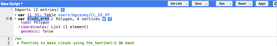
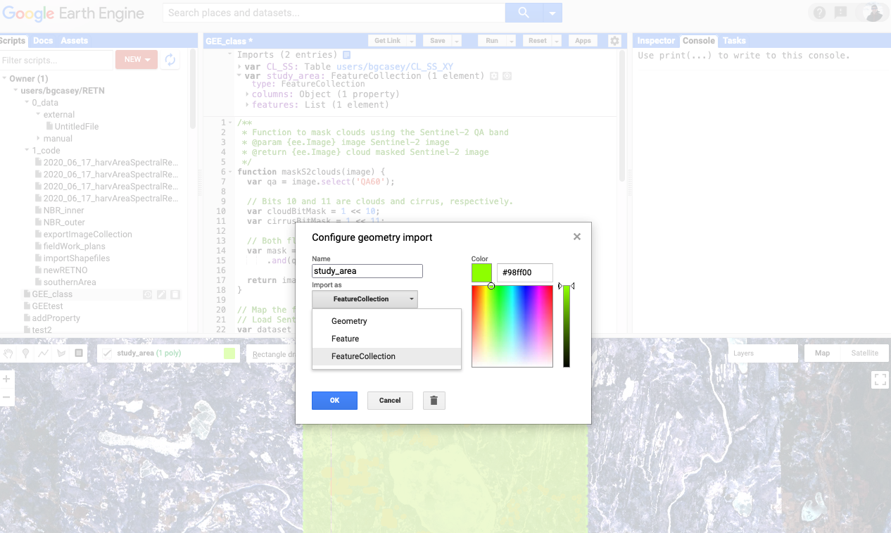
Change the format from geometry to feature collection. This will make it easier to apply styles. Run your cursor over the “study area” label at the top of your map viewer and click the cog icon to edit layer properties. Under Import as select FeatureCollection
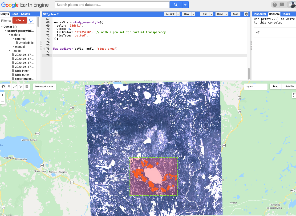
In the code editor, apply styles to the new feature and click run.
var saVis = study_area.style({
  color: '93df41',
  width: 4,
  fillColor: 'ff475750',  // with alpha set for partial transparency
  lineType: 'dotted',
});


Map.addLayer(saVis, null, 'study area')
2.4 Filter image collection
Before selecting data to extract it is important to consider what spatial and temporal resolution you want as well as the desired spectral bands. You can filter the image collection accordingly. First, comment out the previous sentinel import code by using the shortcut `command’ /
We’ll then re-import the image collection and apply the following filters:
- filter by meta data. Here you can filter by meta data values corresponding to percentage of cloud cover. To view all metadata that you can filter your image collection, go to Sentinal-2, Level 1C and click on the Image Properties tab.
- filter by date
- filter by geometry
var s2 = ee.ImageCollection("COPERNICUS/S2");
// Filter by metadata. Here we want cloud cover of less than 30%
var filtered1 = s2.filter(ee.Filter.lt('CLOUDY_PIXEL_PERCENTAGE', <30))
// Filter by date. Here will only use images in the summer season of 2020
var filtered2 = s2.filter(ee.Filter.date('2020-06-01', '2020-09-01'))
// Filter by location. Here we will filter by the study area geometry
var filtered3 = s2.filter(ee.Filter.bounds(study_area))
// Instead of applying filters one after the other, we can 'chain' them
// Use the . notation to apply all the filters together
var filtered = s2.filter(ee.Filter.lt('CLOUDY_PIXEL_PERCENTAGE', 30))
.filter(ee.Filter.date('2019-01-01', '2020-01-01'))
.filter(ee.Filter.bounds(study_area))
print(filtered.size())
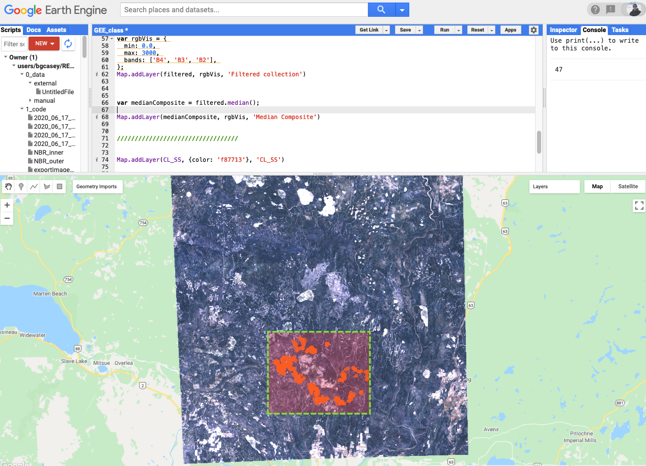
var rgbVis = {
min: 0.0,
max: 3000,
bands: ['B4', 'B3', 'B2'],
};
Map.addLayer(filtered, rgbVis, 'Filtered')