Chapter 2 Solving Equations
2.1 The Bisection Method
bisect <- function(a, b, f, tol = 1e-8) {
    while(abs(b - a) > 2*tol) {
        c = (a+b)/2
        if (f(c) == 0) return(c)
        if (f(a)*f(c) < 0) b = c
        else a = c
    }

    return(c)
}

f <- function(x) x^2 - 5*x - 2
(zero <- bisect(-100, 100, f))
## [1] -0.3722813f(zero)## [1] 5.57046e-08f <- function(x) exp(-x) - x^3 + sin(x)
(zero <- bisect(-100, 100, f))## [1] 1.068532f(zero)## [1] 3.235999e-082.2 Fixed-Point Iteration
fixedpoint <- function(x, f, maxiter = 50, tol = 1e-8) {
    for(i in 1:maxiter) {
        x0 = f(x)
        if (x0 == Inf) return('Diverged')
        if (abs(x0 - x) < 2*tol) return(x0)
        x = x0
    }
    return(x0)
}
f <- function(x) cos(x)
(zero <- fixedpoint(0, f))
## [1] 0.7390851f(zero)## [1] 0.7390851f <- function(x) x^2 - x
(zero <- fixedpoint(5, f))## [1] "Diverged"2.3 Limits of Accuracy
2.4 Newton’s Method
newtonsmethod <- function(x, f, fprime, maxiter = 50, tol = 1e-8) {
    for(i in 1:maxiter) {
        x0 = x - f(x)/fprime(x)
        if(abs(x - x0) < tol) return(x0)
        x = x0
    }
    return(x0)
}

f <- function(x) cos(x) + x^7
fprime <- function(x) -sin(x) + 7*x^6
(zero <- newtonsmethod(10, f, fprime))
## [1] -0.9292731f(zero)## [1] 02.5 Root-Finding Without Derivatives
2.5.1 Secant Method
secantmethod <- function(x0, x1, f, maxiter = 50, tol = 1e-8) {

    for(i in 1:maxiter) {
        xnext = x1 - f(x1)*(x1-x0)/(f(x1)-f(x0))
        x0 = x1
        x1 = xnext
        if (abs(x1 - x0) < tol) return(x1)
    }
    return(x1)
}
f <- function(x) x^2 - x^3 + x - cos(x)
(zero <- secantmethod(0, 1, f))
## [1] 0.6489067f(zero)## [1] -1.110223e-162.5.2 Method of False Position
methodfalseposition <- function(a, b, f, maxiter = 50, tol = 1e-8) {
    i <- 0
    while(abs(b - a) > tol & i < maxiter) {
        c = (b*f(a) - a*f(b))/(f(a) - f(b))
        if (f(c) == 0) return(c)
        if(f(a)*f(c) < 0) b = c
        else a = c
        i <- i+1
    }
    return(c)
}

f <- function(x) x^2 - 3*x - 3
(zero <- methodfalseposition(-10, 10, f))
## [1] 3.791288f(zero)## [1] 3.119283e-112.5.3 Inverse Quadratic Interpolation
invquadint <- function(x1, x2, x3, f, maxiter = 50, tol = 1e-8) {
    for(i in 1:maxiter) {
        q = f(x1)/f(x2)
        r = f(x3)/f(x2)
        s = f(x3)/f(x1)

        xnext = x3 - (r*(r-q)*(x3 - x2) + (1 - r)*s*(x3 - x1))/((q - 1)*(r-1)*(s-1))
        x1 = x2
        x2 = x3
        x3 = xnext
        if (abs(x3 - x2) < tol) return(x3)
    }
    return(x3)
}

f <- function(x) x^2 - x - 3
(zero <- invquadint(-5, 0, 5, f))
## [1] 2.302776f(zero)## [1] -1.332268e-152.5.4 Brent’s Method
brent <- function(a, b, f, maxiter = 50, tol = 1e-8) {
    if (!f(a) * f(b) < 0) stop('f(a) and f(b) must have opposite signs')
    for(i in 1:maxiter) {

    }
}
2.6 Reality Check: Kinematics of the Stewart Platform
A Stewart platform consists of six variable length struts, or prismatic joints, supporting a payload. Prismatic joints operate by changing the length of the strut, usually pneumatically or hydraulically. As a six-degree-of-freedom robot, the Stewart platform can be placed at any point and inclination in three-dimensional space that is within its reach.
To simplify matters, the project concerns a two-dimensional version of the Stewart platform. It will model a manipulator composed of a triangular platform in a fixed plane controlled by three struts, as shown in Figure 1.14. The inner triangle represents the planar Stewart platform whose dimensions are defined by the three lengths \(L_1\),\(L_2\), and \(L_3\). Let \(\gamma\) denote the angle across from side \(L_1\). The position of the platform is controlled by the three numbers \(p_1\),\(p_2\), and \(p_3\), the variable lengths of the three struts.
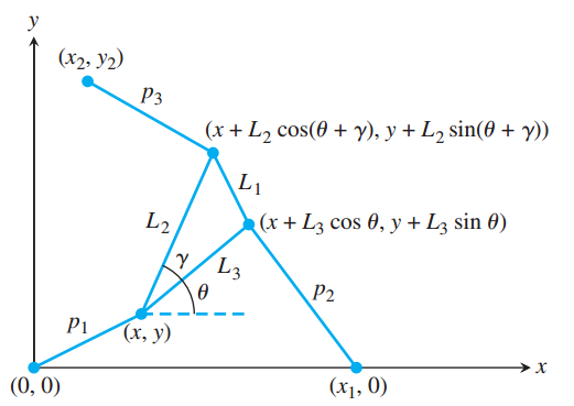
Finding the position of the platform, given the three strut lengths, is called the forward, or direct, kinematics problem for this manipulator. Namely, the problem is to compute (x, y) and \(\theta\) for each given \(p_1\),\(p_2\),\(p_3\). Since there are three degrees of freedom, it is natural to expect three numbers to specify the position. For motion planning, it is important to solve this problem as fast as possible, often in real time. Unfortunately, no closed-form solution of the planar Stewart platform forward kinematics problem is known.
The best current methods involve reducing the geometry of Figure 1.14 to a single equation and solving it by using one of the solvers explained in this chapter. Your job is to complete the derivation of this equation and write code to carry out its solution. Simple trigonometry applied to Figure 1.14 implies the following three equations:
- \(p^2_1 = x^2 + y^2\)
- \(p^2_2 = (x + A_2)^2 + (y + B_2)^2\)
- \(p^2_3 = (x + A_3)^2 + (y + B_3)^2\). (1.38)
In these equations,
- \(A_2 = L_3cos\theta - x_1\)
- \(B_2 = L_3 sin\theta\)
- \(A_3 = L_2cos(\theta + \gamma) - x_2 = L_2[cos\theta cos\gamma - sin\theta sin\gamma] - x_2\)
- \(B_3 = L_2 sin(\theta + \gamma) - y_2 = L_2[cos\theta sin\gamma + sin\theta cos\gamma] - y_2\)
Note that (1.38) solves the inverse kinematics problem of the planar Stewart platform, which is to find \(p_1\), \(p_2\), \(p_3\), given x, y, \(\theta\). Your goal is to solve the forward problem, namely, to find x, y, \(\theta\), given \(p_1\), \(p_2\), \(p_3\).
Multiplying out the last two equations of (1.38) and using the first yields
\(p^2_2 = x^2 + y^2 + 2A_2x + 2B_2y + A^2_2 + B^2_2 = p^2_1 + 2A_2x + 2B_2y + A^2_2 + B^2_2\)
\(p^2_3 = x^2 + y^2 + 2A_3x + 2B_3y + A^2_3 + B^2_3 = p^2_1 + 2A_3x + 2B_3y + A^2_3 + B^2_3\),
which can be solved for x and y as
\(x = \frac{N_1}{D} = \frac{B_3(p^2_2 - p^2_1 - A^2_2 - B^2_2) - B_2(p^2_3 - p^2_1 - A^2_3 - B^2_3)}{2(A_2B_3 - B_2A_3)}\)
\(y = \frac{N_2}{D} = \frac{-A_3(p^2_2 - p^2_1 - A^2_2 - B^2_2) + A_2(p^2_3 - p^2_1 - A^2_3 - B^2_3)}{2(A_2B_3 - B_2A_3)}\)
as long as \(D = 2(A_2B_3 - B_2A_3) \neq 0\).
Substituting these expressions for x and y into the first equation of (1.38), and multiplying through by \(D^2\), yields one equation, namely,
- \(f = N^2_1 + N^2_2 - p^2_1D^2 = 0\)
in the single unknown \(\theta\). (Recall that \(p_1,p_2,p_3,L_1,L_2,L_3,\gamma,x_1,x_2,y_2\) are known.) If the roots of \(f(\theta)\) can be found, the corresponding x- and y- values follow immediately from (1.39).
Note that \(f(\theta)\) is a polynomial in \(sin(\theta)\) and \(cos(\theta)\), so, given any root \(\theta\), there are other roots \(\theta + 2\pi k\) that are equivalent for the platform. For that reason, we can restrict attention to \(\theta\) in \([-\pi, \pi]\). It can be shown that \(f(\theta)\) has at most six roots in that interval.
2.6.1 Suggested Activities
Write a function for \(f(\theta)\). The parameters \(L_1, L_2, L_3, \gamma, x_1, x_2, y_2\) are fixed constants and the strut lengths \(p_1, p_2, p_3\) will be known for a given pose. To test your code set the parameters \(L_1 = 2, L_2 = L_3 = \sqrt2, \gamma = \pi/2, p_1=p_2=p_3=\sqrt5\). Then substituting \(\theta = -\pi /4\) or \(\theta = \pi /4\) should make \(f(\theta) = 0\)