6 Item Response Theory
In this chapter, we present an example of using R to conduct an item response theory analysis (IRT) of the Academic Motivation Scale (AMS) included in a compendium of scales designed for use by school social workers. The Community and Youth Collaborative Institute School Experience Surveys http://cayci.osu.edu/surveys/) resource makes available various scales designed for elementary, middle, and high school students, teachers and staff, and parents and caregivers. The scales are marketed as valid and reliable measures of constructs that are important for needs assessments, program planning, and program evaluations in school settings.
For this analysis, we use the R mirt package to fit and assess a graded response model to the six-item AMS. The items are:
- I have a positive attitude toward school
- I feel I have made the most of my school experiences so far
- I like the challenges of learning new things in school
- I am confident in my ability to manage my school work
- I feel my school experience is preparing me well for adulthood
- I have enjoyed my school experience so far
The response categories are Strongly disagree, Disagree, Can’t decide, Agree, and Strongly agree.
First, we load libraries and data as follows:
# Load the mirt library
library(mirt)
library(knitr)
library(dplyr)
The data used in this study came from 3,221 seventh grade students in seventeen school districts in a large mid-western urban county. We load the data file with these commands:
##Load Data
data <- read.csv("motivation.csv", header=TRUE)
scale <-(data[,1:6])
head(scale, 3)
## Item.1 Item.2 Item.3 Item.4 Item.5 Item.6
## 1 4 4 3 4 4 4
## 2 5 2 3 2 5 5
## 3 5 4 4 4 5 56.1 Fit and assess model
As noted, we used the R mirt package to fit a graded response model (the recommended model for ordered polytomous response data) using a full-information maximum likelihood fitting function. In addition, we assessed model fit using an index, M2, which is specifically designed to assess the fit of item response models for ordinal data. We used the M2-based root mean square error of approximation as the primary fit index. We also used the standardized root mean square residual (SRMSR) and comparative fit index (CFI) to assess adequacy of model fit.
6.1.1 Model fit
mod1 <- (mirt(scale, 1, verbose = FALSE, itemtype = 'graded', SE = TRUE))M2(mod1, type = "C2", calcNULL = FALSE)## M2 df p RMSEA RMSEA_5 RMSEA_95 SRMSR TLI CFI
## stats 89.955 9 1.6653e-15 0.052853 0.043236 0.063035 0.030703 0.98185 0.98911The obtained RMSEA value = .053 (95% CI[.043, .063]) and SRMSR value = .031 suggest that data fit the model reasonably well using suggested cutoff values of RMSEA <= .06 and SRMSR <= .08 as suggested guidelines for assessing fit. The CFI = .945 was just below a recommended .95 threshold (although it would be .95 rounded).
6.1.2 Item fit
A second area of of interest is to assess how well each item fits the model. For this assessment, we use a recommended index–S-X2. The mirt implementation of S-X2 computes an RMSEA value which can be used to assess degree of item fit. Values less than .06 are considered evidence of adequate fit.
itemfit(mod1)## item S_X2 df.S_X2 RMSEA.S_X2 p.S_X2
## 1 Item.1 69.518 49 0.011 0.028
## 2 Item.2 90.946 52 0.015 0.001
## 3 Item.3 85.472 51 0.014 0.002
## 4 Item.4 87.002 50 0.015 0.001
## 5 Item.5 81.205 51 0.014 0.005
## 6 Item.6 54.692 48 0.007 0.235All of the RMSEA values are less than .06 indicating that the items had adequate fit with the model.
Once we established the adequacy of model and item fit, we then computed item parameters. IRT provides two assessments of item-latent trait relationships. The IRT parameterization generates discrimination and location parameters. The factor analysis parameterization generates factor loadings and communlaities.
6.1.3 IRT parameters:
# IRT parameters
coef(mod1, IRTpars = TRUE, simplify = TRUE)
## $items
## a b1 b2 b3 b4
## Item.1 1.865 -2.516 -1.591 -0.647 1.159
## Item.2 1.466 -3.147 -1.759 -0.695 1.160
## Item.3 1.443 -2.755 -1.693 -0.556 1.110
## Item.4 1.569 -3.359 -2.204 -1.084 0.838
## Item.5 1.680 -2.742 -1.891 -0.853 0.671
## Item.6 1.918 -2.328 -1.634 -0.757 0.774
##
## $means
## F1
## 0
##
## $cov
## F1
## F1 1The estimated IRT parameters are shown above. The values of the slope (a-parameters) parameters ranged from 1.44 to 1.92. A slope parameter is a measure of how well an item differentiates respondents with different levels of the latent trait. Larger values, or steeper slopes, are better at differentiating theta. A slope also can be interpreted as an indicator of the strength of a relationship between and item and latent trait, with higher slope values corresponding to stronger relationships. Item 6 was the most discriminating items with a slope estimate of 1.92 while Item 3 was the least discriminating item with a slope estimate of 1.44.
Three location parameters (b-parameters) also are listed for each item. Location parameters are interpreted as the value of theta that corresponds to a .5 probability of responding at or above that location on an item. There are m-1 location parameters where m refers to the number of response categories on the response scale. The location parameters indicate that responses covered a wide range of the latenet trait.
6.1.4 Factor analysis parameters:
# Factor loadings
summary(mod1)
## F1 h2
## Item.1 0.739 0.546
## Item.2 0.653 0.426
## Item.3 0.647 0.418
## Item.4 0.678 0.459
## Item.5 0.702 0.493
## Item.6 0.748 0.560
##
## SS loadings: 2.902
## Proportion Var: 0.484
##
## Factor correlations:
##
## F1
## F1 1Factor loadings can be interpreted as a strength of the relationship between an item and the latent variable (F1). The Communalities (h2) are squared factor loadings and are interpreted as the variance accounted for in an item by the latent trait. All of the items had a substantive relationship (loadings > .50) with the latent trait.
6.2 IRT Plots
A strength of IRT is the ability to visually examine item and scale characteristics using various plots. These plots display how each item and the total scale relate to the latent trait across trait values. This capacity is where IRT methods have an advantage over classical test methods and CFA/SEM methods.
In this example, we explore item and scale latent trait relationships using:
- Category characteristic curves
- Item information curves
- Scale information and conditional standard error curves
- Conditional reliability curve
- Scale characteristic curve
6.2.1 Category characteristic curves
It often is of interest to examine the probabilities of responding to specific categories in an item’s response scale. These probabilities are graphically displayed in the category response curves (CRCs) shown below.
plot(mod1, type='trace', which.item = c(1,2,3,4,5,6), facet_items=T,
as.table = TRUE, auto.key=list(points=F, lines=T, columns=4, space = 'top', cex = .8),
theta_lim = c(-3, 3),
main = "")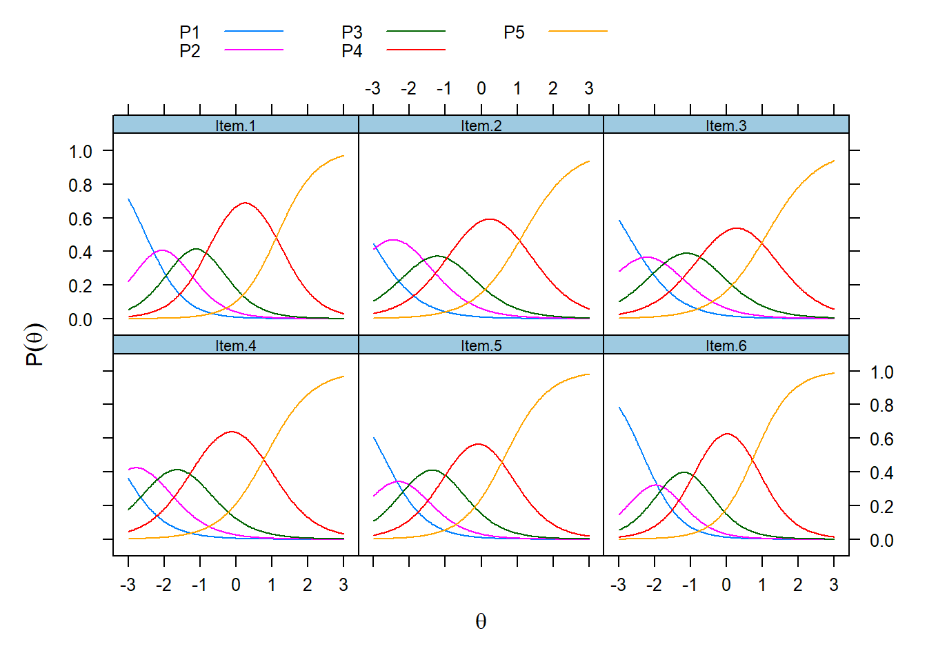 Each symmetrical curve represents the probability of endorsing a response category (P1 = ‘Strongly disagree,’ P2 = ‘Disagree”, P3 = “Can’t decide,” P4 = “Agree,” and P5 = "Strongly agree). These curves have a functional relationship with theta; As theta increases, the probability of endorsing a category increases and then decreases as responses transition to the next higher category. The CRCs indicate that the response categories cover a wide range of theta.
6.2.2 Item information curves
Information is a statistical concept that refers to the ability of an item to accurately estimate scores on theta. Item level information clarifies how well each item contributes to score estimation precision with higher levels of information leading to more accurate score estimates.
plot(mod1, type='infotrace', which.item = c(1,2,3,4,5,6), facet_items=T,
     as.table = TRUE, auto.key=list(points=F, lines=T, columns=1, space = 'right', cex = .8),
              theta_lim = c(-3, 3),
     main="")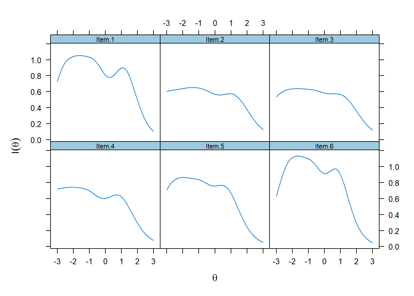
In polytomous models, the amount of information an item contributes depends on its slope parameter—–the larger the parameter, the more information the item provides. Further, the farther apart the location parameters (b1, b2, b3, b4), the more information the item provides. Typically, an optimally informative polytomous item will have a large location and broad category coverage (as indicated by location parameters) over theta.
Information functions are best illustrated by the item information curves for each item as displayed above. These curves show that item information is not a static quantity, rather, it is conditional on levels of theta. The relationship between slopes and information is illustrated here. Item 3 had the lowest slope and is, therefore, the least informative item.On the other hand, Item 9 had the highest slope and provides the highest amount of statistical information. Items tended to provide the most information between -2.5 to + 1 theta range. The “wavy” form of the curves reflects the fact that item information is a composite of category information, that is, each category has an information function which is then combined to form the item information function.
6.2.3 Scale information and conditional standard errors
One particularly helpful IRT capacity is that information for individual items can be summed to form a scale information function. A scale information function is a summary of how well items, overall, provide statistical information about the latent trait. Further, scale information values can be used to compute conditional standard errors which indicate how precisely scores can be estimated across different values of theta.
plot(mod1, type = 'infoSE', theta_lim = c(-3, 3),
     main="")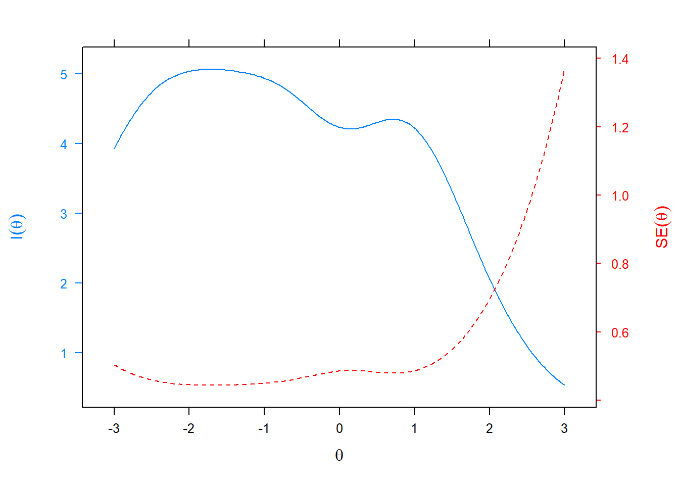
The relationship between scale information and conditional standard errors is illustrated above. The solid blue line represents the scale information function. The overall scale provided the most information in the range -2.5 to + 1. The red line provides a visual reference about how estimate precision varies across theta with smaller values corresponding to better estimate precision. Because conditional standard errors mathematically mirror the scale information curve, estimated score precision was best in the -2.5 to + 1 theta range.
6.2.4 Conditional reliability
IRT approaches the concept of scale reliability differently than the traditional classical test theory approach using coefficient alpha or omega. The CTT approach assumes that reliability is based on a single value that applies to all scale scores.
plot(mod1, type = 'rxx', theta_lim = c(-3, 3),
     main="" )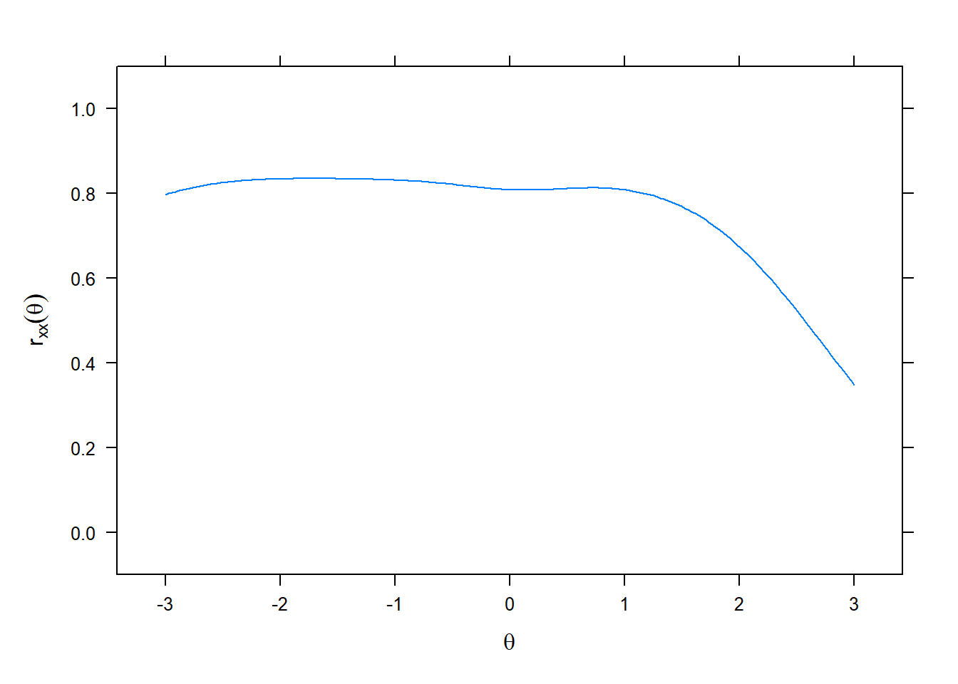
The concept of conditional reliability is illustrated in the above. This curve is mathematically related to both scale information and conditional standard errors through simple transformations. Because of this relationship, score estimates are most reliable in the -2.5 to + 1 theta range.
It also is possible to compute a single IRT reliability estimate. The marginal reliability for the AMS = .80.
marginal_rxx(mod1)## [1] 0.806576.2.5 Scale characteristic curve
As a next step, we used model parameters to generate estimates of student theta scores. These scores are referred to as person parameters in IRT (they are called factor scores in CFA). We used a latent trait scoring procedure called expected a posteriori (EAP) estimation to generate the scores. Keep in mind the estimates are in the theta (standard normal) metric so they are z-like scores. Thus, IRT model-based scores have favorable properties that improve on a summed score approach. First, model-based scores reflect the impacts of parameter estimates obtained from the IRT model used. As a result, because they are weighted by item parameters, theta score estimates often show more variability than summed scores. They also can be interpreted in the standard normal framework; because they are given in a standard normal metric, we can use our knowledge of the standard normal distribution to make score comparisons across individuals. For example, someone with a theta score of 1.0 is one standard deviation above average and we can expect that 84% of the sample to have lower scores and 16% to have higher scores. Other comparisons of interest based on standard normal characteristics are possible.
Once model-based theta score estimates are computed, it often is of interest to transform those estimates into the original scale metric. A scale characteristic function provides a means of transforming estimated theta scores to expected true scores in the original scale metric. This transformation back into the original scale metric provides a more familiar frame of reference for interpreting scores. In this study, expected true scores refer to scores on the AMS scale metric (6 to 30) that are expected as a function of estimated student theta scores.
plot(mod1, type = 'score', theta_lim = c(-3, 3), main = "")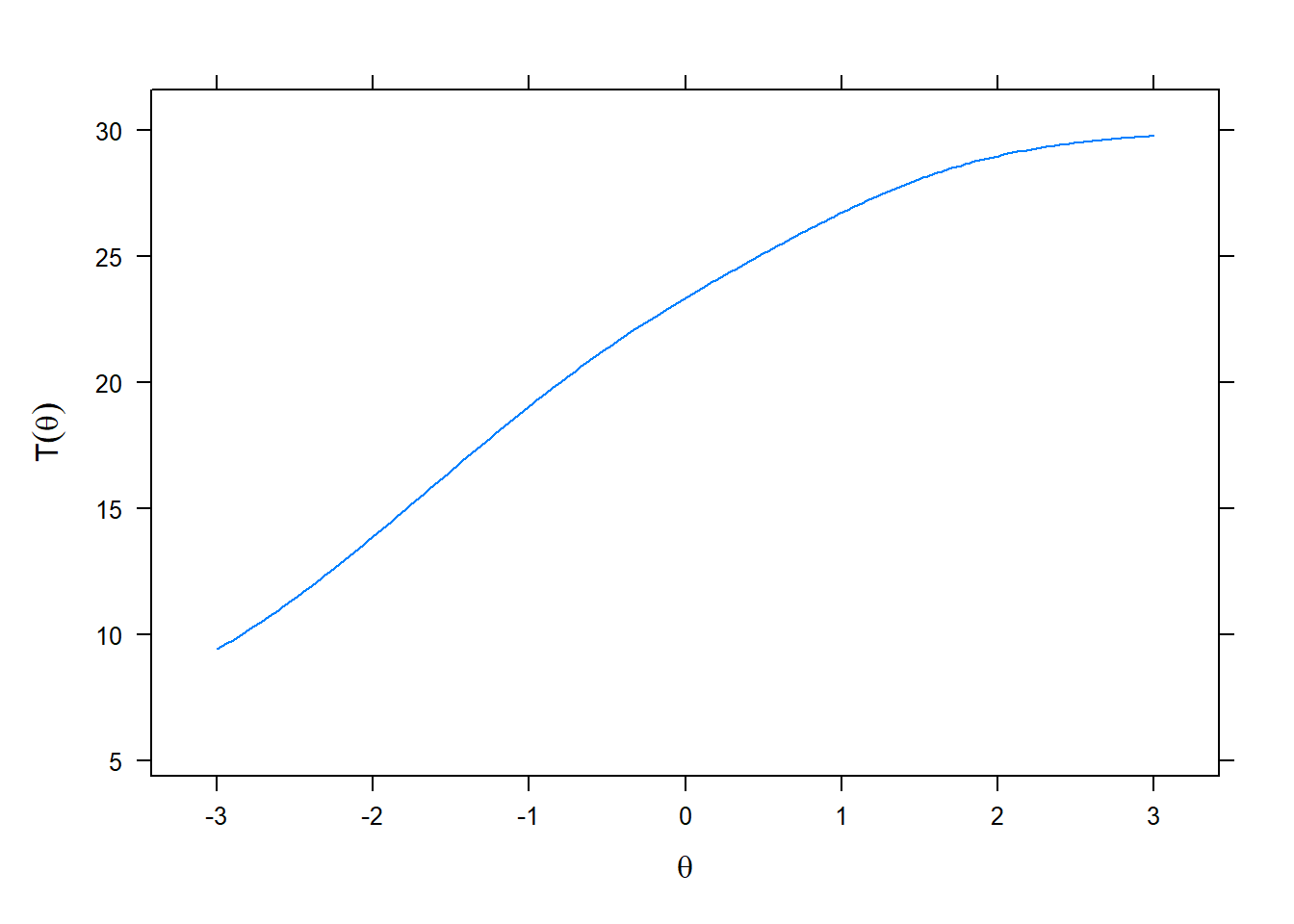
The scale characteristic function can be graphically displayed as shown above. It has a straightforward use; for any given estimated theta score we can easily find a corresponding expected true score in the summed scale score metric. These true score transformations often are of interest in practical situations where scale users are not familiar with theta scores. Also, true score estimates can be used in other important statistical analyses and are often improvements over traditional summed scores.
6.3 Summary
The overall conclusion we reached about the AMS based on the IRT analysis is that the scale is a psychometrically sound measure of academic motivation. Both model fit and item fit indexes were acceptable. Each item had a substantive link to the latent trait. Items had slope parameters indicating they were able to differentiate respondents with different levels of the future orientation. All-in-all we can recommend the AMS for use by school social workers.