12 Tidy data
12.1 Introduction
“Happy families are all alike; every unhappy family is unhappy in its own way.” –– Leo Tolstoy
“Tidy datasets are all alike, but every messy dataset is messy in its own way.” –– Hadley Wickham
In this chapter, you will learn a consistent way to organise your data in R, an organisation called tidy data. Getting your data into this format requires some upfront work, but that work pays off in the long term. Once you have tidy data and the tidy tools provided by packages in the tidyverse, you will spend much less time munging data from one representation to another, allowing you to spend more time on the analytic questions at hand.
This chapter will give you a practical introduction to tidy data and the accompanying tools in the tidyr package. If you’d like to learn more about the underlying theory, you might enjoy the Tidy Data paper published in the Journal of Statistical Software, http://www.jstatsoft.org/v59/i10/paper.
12.1.1 Prerequisites
In this chapter we’ll focus on tidyr, a package that provides a bunch of tools to help tidy up your messy datasets. tidyr is a member of the core tidyverse.
library(tidyverse)12.2 Tidy data
You can represent the same underlying data in multiple ways. The example below shows the same data organised in four different ways. Each dataset shows the same values of four variables country, year, population, and cases, but each dataset organises the values in a different way.
table1
#> # A tibble: 6 × 4
#>       country  year  cases population
#>         <chr> <int>  <int>      <int>
#> 1 Afghanistan  1999    745   19987071
#> 2 Afghanistan  2000   2666   20595360
#> 3      Brazil  1999  37737  172006362
#> 4      Brazil  2000  80488  174504898
#> 5       China  1999 212258 1272915272
#> 6       China  2000 213766 1280428583
table2
#> # A tibble: 12 × 4
#>       country  year       type     count
#>         <chr> <int>      <chr>     <int>
#> 1 Afghanistan  1999      cases       745
#> 2 Afghanistan  1999 population  19987071
#> 3 Afghanistan  2000      cases      2666
#> 4 Afghanistan  2000 population  20595360
#> 5      Brazil  1999      cases     37737
#> 6      Brazil  1999 population 172006362
#> # ... with 6 more rows
table3
#> # A tibble: 6 × 3
#>       country  year              rate
#> *       <chr> <int>             <chr>
#> 1 Afghanistan  1999      745/19987071
#> 2 Afghanistan  2000     2666/20595360
#> 3      Brazil  1999   37737/172006362
#> 4      Brazil  2000   80488/174504898
#> 5       China  1999 212258/1272915272
#> 6       China  2000 213766/1280428583

# Spread across two tibbles
table4a  # cases
#> # A tibble: 3 × 3
#>       country `1999` `2000`
#> *       <chr>  <int>  <int>
#> 1 Afghanistan    745   2666
#> 2      Brazil  37737  80488
#> 3       China 212258 213766
table4b  # population
#> # A tibble: 3 × 3
#>       country     `1999`     `2000`
#> *       <chr>      <int>      <int>
#> 1 Afghanistan   19987071   20595360
#> 2      Brazil  172006362  174504898
#> 3       China 1272915272 1280428583
These are all representations of the same underlying data, but they are not equally easy to use. One dataset, the tidy dataset, will be much easier to work with inside the tidyverse.
There are three interrelated rules which make a dataset tidy:
- Each variable must have its own column.
- Each observation must have its own row.
- Each value must have its own cell.
Figure 12.1 shows the rules visually.
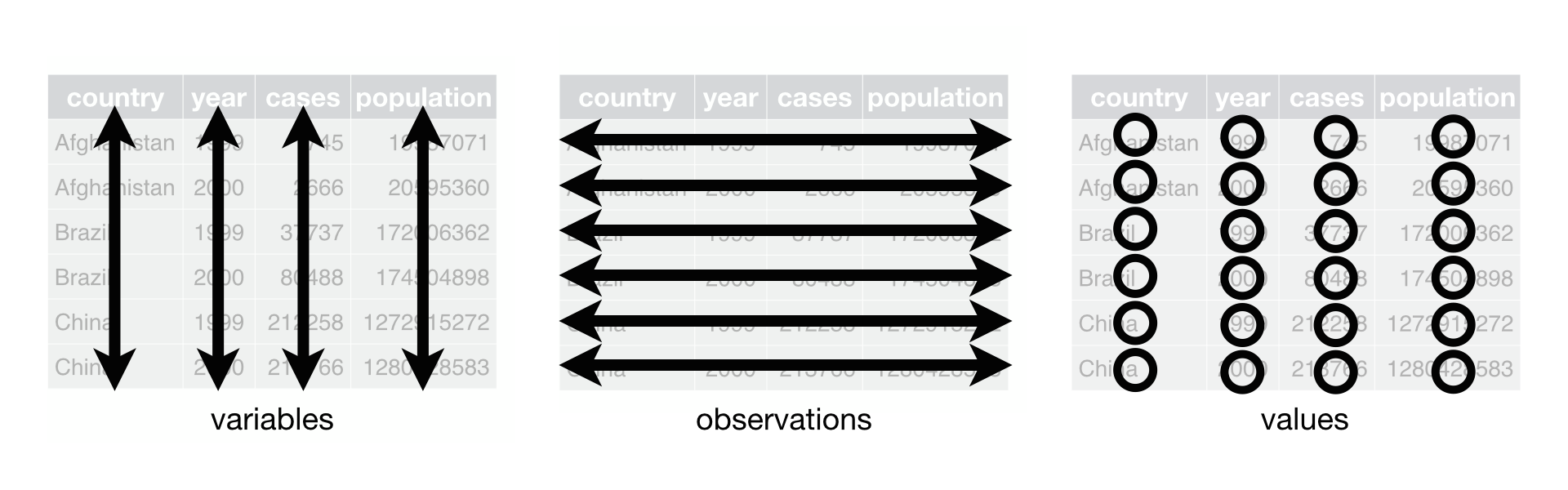
Figure 12.1: Following three rules makes a dataset tidy: variables are in columns, observations are in rows, and values are in cells.
These three rules are interrelated because it’s impossible to only satisfy two of the three. That interrelationship leads to an even simpler set of practical instructions:
- Put each dataset in a tibble.
- Put each variable in a column.
In this example, only table1 is tidy. It’s the only representation where each column is a variable.
Why ensure that your data is tidy? There are two main advantages:
There’s a general advantage to picking one consistent way of storing data. If you have a consistent data structure, it’s easier to learn the tools that work with it because they have an underlying uniformity.
There’s a specific advantage to placing variables in columns because it allows R’s vectorised nature to shine. As you learned in mutate and summary functions, most built-in R functions work with vectors of values. That makes transforming tidy data feel particularly natural.
dplyr, ggplot2, and all the other packages in the tidyverse are designed to work with tidy data. Here are a couple of small examples showing how you might work with table1.
# Compute rate per 10,000
table1 %>%
  mutate(rate = cases / population * 10000)
#> # A tibble: 6 × 5
#>       country  year  cases population  rate
#>         <chr> <int>  <int>      <int> <dbl>
#> 1 Afghanistan  1999    745   19987071 0.373
#> 2 Afghanistan  2000   2666   20595360 1.294
#> 3      Brazil  1999  37737  172006362 2.194
#> 4      Brazil  2000  80488  174504898 4.612
#> 5       China  1999 212258 1272915272 1.667
#> 6       China  2000 213766 1280428583 1.669

# Compute cases per year
table1 %>%
  count(year, wt = cases)
#> # A tibble: 2 × 2
#>    year      n
#>   <int>  <int>
#> 1  1999 250740
#> 2  2000 296920

# Visualise changes over time
library(ggplot2)
ggplot(table1, aes(year, cases)) +
  geom_line(aes(group = country), colour = "grey50") +
  geom_point(aes(colour = country))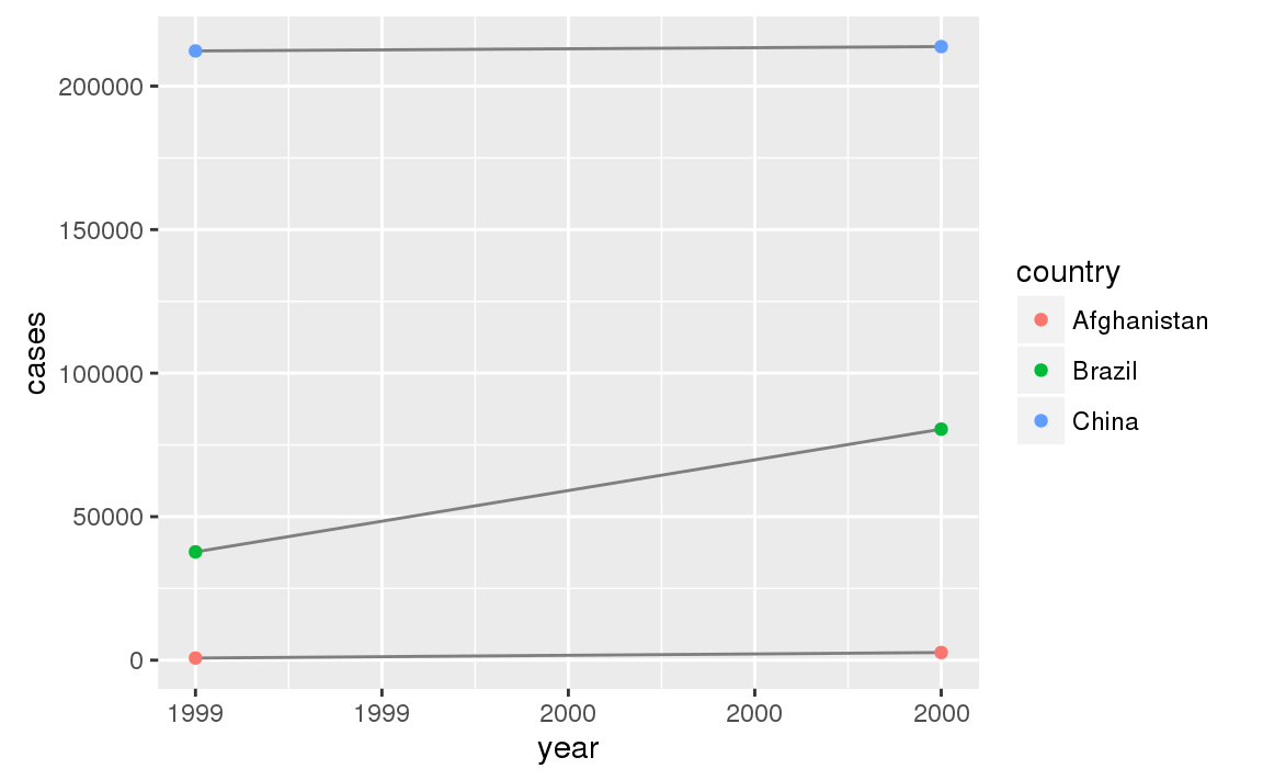
12.2.1 Exercises
Using prose, describe how the variables and observations are organised in each of the sample tables.
Compute the
ratefortable2, andtable4a+table4b. You will need to perform four operations:- Extract the number of TB cases per country per year.
- Extract the matching population per country per year.
- Divide cases by population, and multiply by 10000.
- Store back in the appropriate place.
Which representation is easiest to work with? Which is hardest? Why?
Recreate the plot showing change in cases over time using
table2instead oftable1. What do you need to do first?
12.3 Spreading and gathering
The principles of tidy data seem so obvious that you might wonder if you’ll ever encounter a dataset that isn’t tidy. Unfortunately, however, most data that you will encounter will be untidy. There are two main reasons:
Most people aren’t familiar with the principles of tidy data, and it’s hard to derive them yourself unless you spend a lot of time working with data.
Data is often organised to facilitate some use other than analysis. For example, data is often organised to make entry as easy as possible.
This means for most real analyses, you’ll need to do some tidying. The first step is always to figure out what the variables and observations are. Sometimes this is easy; other times you’ll need to consult with the people who originally generated the data. The second step is to resolve one of two common problems:
One variable might be spread across multiple columns.
One observation might be scattered across multiple rows.
Typically a dataset will only suffer from one of these problems; it’ll only suffer from both if you’re really unlucky! To fix these problems, you’ll need the two most important functions in tidyr: gather() and spread().
12.3.1 Gathering
A common problem is a dataset where some of the column names are not names of variables, but values of a variable. Take table4a: the column names 1999 and 2000 represent values of the year variable, and each row represents two observations, not one.
table4a
#> # A tibble: 3 × 3
#>       country `1999` `2000`
#> *       <chr>  <int>  <int>
#> 1 Afghanistan    745   2666
#> 2      Brazil  37737  80488
#> 3       China 212258 213766
To tidy a dataset like this, we need to gather those columns into a new pair of variables. To describe that operation we need three parameters:
The set of columns that represent values, not variables. In this example, those are the columns
1999and2000.The name of the variable whose values form the column names. I call that the
key, and here it isyear.The name of the variable whose values are spread over the cells. I call that
value, and here it’s the number ofcases.
Together those parameters generate the call to gather():
table4a %>%
  gather(`1999`, `2000`, key = "year", value = "cases")
#> # A tibble: 6 × 3
#>       country  year  cases
#>         <chr> <chr>  <int>
#> 1 Afghanistan  1999    745
#> 2      Brazil  1999  37737
#> 3       China  1999 212258
#> 4 Afghanistan  2000   2666
#> 5      Brazil  2000  80488
#> 6       China  2000 213766
The columns to gather are specified with dplyr::select() style notation. Here there are only two columns, so we list them individually. Note that “1999” and “2000” are non-syntactic names so we have to surround them in backticks. To refresh your memory of the other ways to select columns, see select.
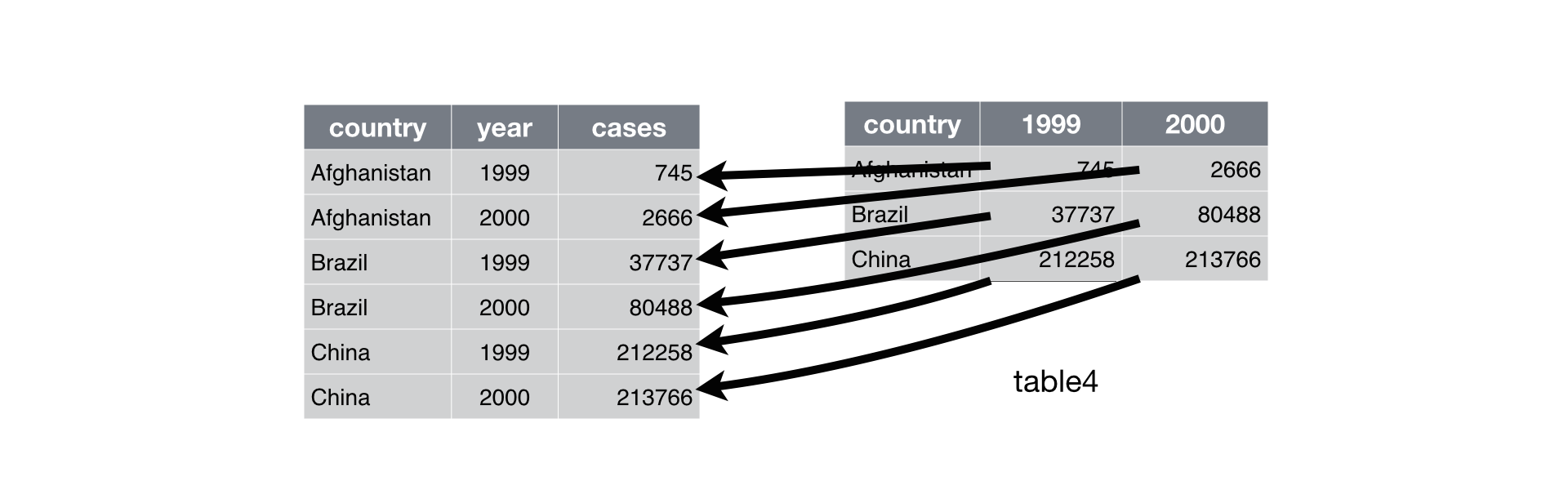
Figure 12.2: Gathering table4 into a tidy form.
In the final result, the gathered columns are dropped, and we get new key and value columns. Otherwise, the relationships between the original variables are preserved. Visually, this is shown in Figure 12.2. We can use gather() to tidy table4b in a similar fashion. The only difference is the variable stored in the cell values:
table4b %>%
  gather(`1999`, `2000`, key = "year", value = "population")
#> # A tibble: 6 × 3
#>       country  year population
#>         <chr> <chr>      <int>
#> 1 Afghanistan  1999   19987071
#> 2      Brazil  1999  172006362
#> 3       China  1999 1272915272
#> 4 Afghanistan  2000   20595360
#> 5      Brazil  2000  174504898
#> 6       China  2000 1280428583
To combine the tidied versions of table4a and table4b into a single tibble, we need to use dplyr::left_join(), which you’ll learn about in relational data.
tidy4a <- table4a %>%
  gather(`1999`, `2000`, key = "year", value = "cases")
tidy4b <- table4b %>%
  gather(`1999`, `2000`, key = "year", value = "population")
left_join(tidy4a, tidy4b)
#> Joining, by = c("country", "year")
#> # A tibble: 6 × 4
#>       country  year  cases population
#>         <chr> <chr>  <int>      <int>
#> 1 Afghanistan  1999    745   19987071
#> 2      Brazil  1999  37737  172006362
#> 3       China  1999 212258 1272915272
#> 4 Afghanistan  2000   2666   20595360
#> 5      Brazil  2000  80488  174504898
#> 6       China  2000 213766 1280428583
12.3.2 Spreading
Spreading is the opposite of gathering. You use it when an observation is scattered across multiple rows. For example, take table2: an observation is a country in a year, but each observation is spread across two rows.
table2
#> # A tibble: 12 × 4
#>       country  year       type     count
#>         <chr> <int>      <chr>     <int>
#> 1 Afghanistan  1999      cases       745
#> 2 Afghanistan  1999 population  19987071
#> 3 Afghanistan  2000      cases      2666
#> 4 Afghanistan  2000 population  20595360
#> 5      Brazil  1999      cases     37737
#> 6      Brazil  1999 population 172006362
#> # ... with 6 more rows
To tidy this up, we first analyse the representation in similar way to gather(). This time, however, we only need two parameters:
The column that contains variable names, the
keycolumn. Here, it’stype.The column that contains values forms multiple variables, the
valuecolumn. Here it’scount.
Once we’ve figured that out, we can use spread(), as shown programmatically below, and visually in Figure 12.3.
spread(table2, key = type, value = count)
#> # A tibble: 6 × 4
#>       country  year  cases population
#> *       <chr> <int>  <int>      <int>
#> 1 Afghanistan  1999    745   19987071
#> 2 Afghanistan  2000   2666   20595360
#> 3      Brazil  1999  37737  172006362
#> 4      Brazil  2000  80488  174504898
#> 5       China  1999 212258 1272915272
#> 6       China  2000 213766 1280428583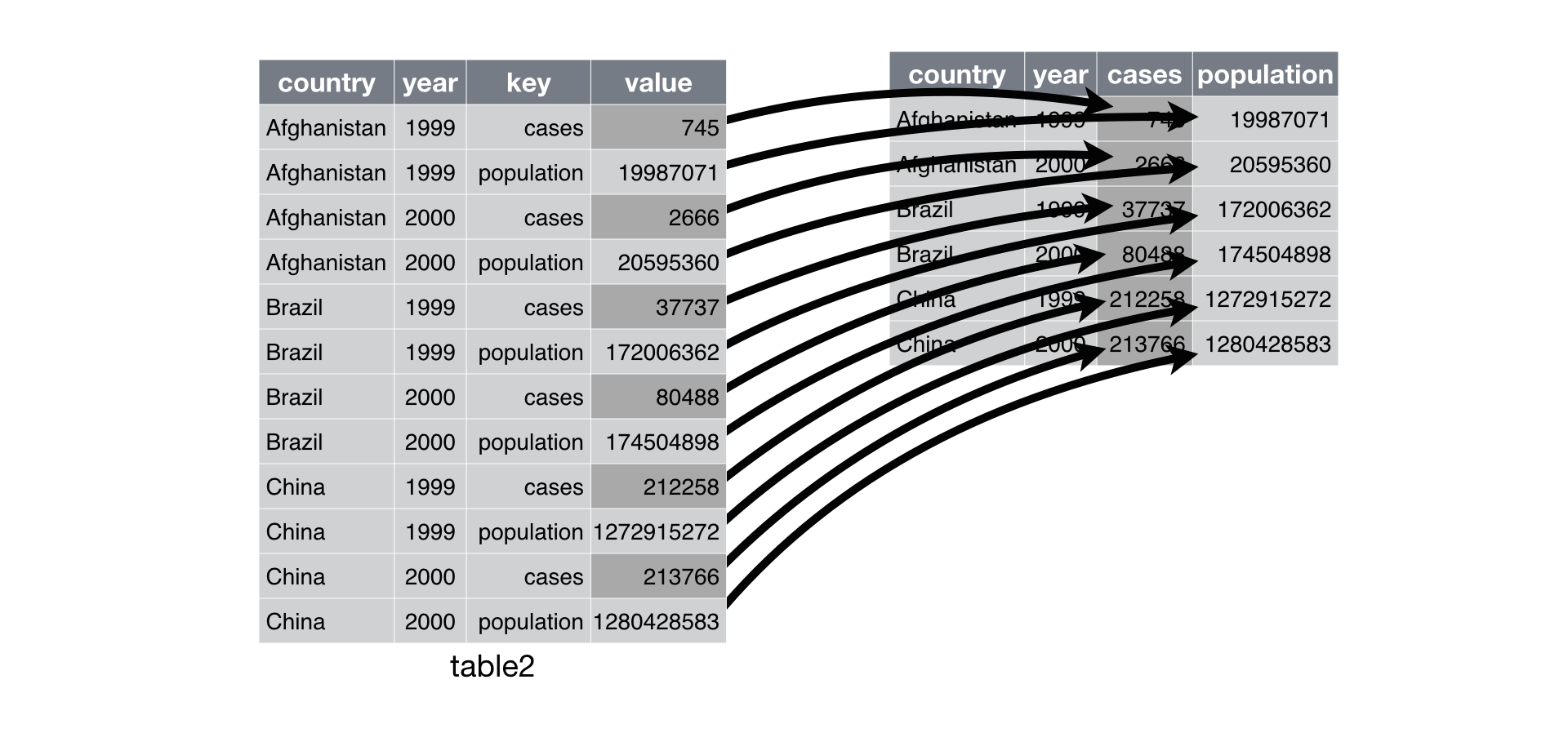
Figure 12.3: Spreading table2 makes it tidy
As you might have guessed from the common key and value arguments, spread() and gather() are complements. gather() makes wide tables narrower and longer; spread() makes long tables shorter and wider.
12.3.3 Exercises
Why are
gather()andspread()not perfectly symmetrical?
Carefully consider the following example:stocks <- tibble( year = c(2015, 2015, 2016, 2016), half = c( 1, 2, 1, 2), return = c(1.88, 0.59, 0.92, 0.17) ) stocks %>% spread(year, return) %>% gather("year", "return", `2015`:`2016`)(Hint: look at the variable types and think about column names.)
Both
spread()andgather()have aconvertargument. What does it do?Why does this code fail?
table4a %>%
  gather(1999, 2000, key = "year", value = "cases")
#> Error in eval(expr, envir, enclos): Position must be between 0 and n
Why does spreading this tibble fail? How could you add a new column to fix the problem?
people <- tribble(
  ~name,             ~key,    ~value,
  #-----------------|--------|------
  "Phillip Woods",   "age",       45,
  "Phillip Woods",   "height",   186,
  "Phillip Woods",   "age",       50,
  "Jessica Cordero", "age",       37,
  "Jessica Cordero", "height",   156
)
Tidy the simple tibble below. Do you need to spread or gather it? What are the variables?
preg <- tribble(
  ~pregnant, ~male, ~female,
  "yes",     NA,    10,
  "no",      20,    12
)
12.4 Separating and uniting
So far you’ve learned how to tidy table2 and table4, but not table3. table3 has a different problem: we have one column (rate) that contains two variables (cases and population). To fix this problem, we’ll need the separate() function. You’ll also learn about the complement of separate(): unite(), which you use if a single variable is spread across multiple columns.
12.4.1 Separate
separate() pulls apart one column into multiple columns, by splitting wherever a separator character appears. Take table3:
table3
#> # A tibble: 6 × 3
#>       country  year              rate
#> *       <chr> <int>             <chr>
#> 1 Afghanistan  1999      745/19987071
#> 2 Afghanistan  2000     2666/20595360
#> 3      Brazil  1999   37737/172006362
#> 4      Brazil  2000   80488/174504898
#> 5       China  1999 212258/1272915272
#> 6       China  2000 213766/1280428583
The rate column contains both cases and population variables, and we need to split it into two variables. separate() takes the name of the column to separate, and the names of the columns to separate into, as shown in Figure 12.4 and the code below.
table3 %>%
  separate(rate, into = c("cases", "population"))
#> # A tibble: 6 × 4
#>       country  year  cases population
#> *       <chr> <int>  <chr>      <chr>
#> 1 Afghanistan  1999    745   19987071
#> 2 Afghanistan  2000   2666   20595360
#> 3      Brazil  1999  37737  172006362
#> 4      Brazil  2000  80488  174504898
#> 5       China  1999 212258 1272915272
#> 6       China  2000 213766 1280428583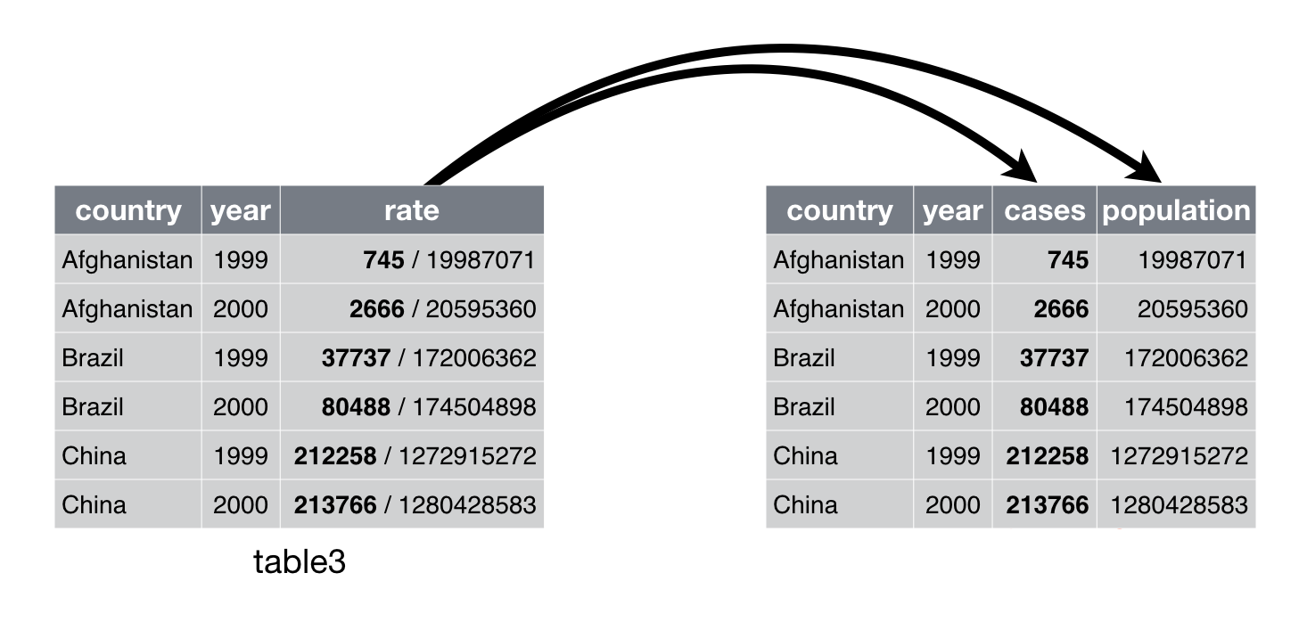
Figure 12.4: Separating table3 makes it tidy
By default, separate() will split values wherever it sees a non-alphanumeric character (i.e. a character that isn’t a number or letter). For example, in the code above, separate() split the values of rate at the forward slash characters. If you wish to use a specific character to separate a column, you can pass the character to the sep argument of separate(). For example, we could rewrite the code above as:
table3 %>%
  separate(rate, into = c("cases", "population"), sep = "/")
(Formally, sep is a regular expression, which you’ll learn more about in strings.)
Look carefully at the column types: you’ll notice that case and population are character columns. This is the default behaviour in separate(): it leaves the type of the column as is. Here, however, it’s not very useful as those really are numbers. We can ask separate() to try and convert to better types using convert = TRUE:
table3 %>%
  separate(rate, into = c("cases", "population"), convert = TRUE)
#> # A tibble: 6 × 4
#>       country  year  cases population
#> *       <chr> <int>  <int>      <int>
#> 1 Afghanistan  1999    745   19987071
#> 2 Afghanistan  2000   2666   20595360
#> 3      Brazil  1999  37737  172006362
#> 4      Brazil  2000  80488  174504898
#> 5       China  1999 212258 1272915272
#> 6       China  2000 213766 1280428583
You can also pass a vector of integers to sep. separate() will interpret the integers as positions to split at. Positive values start at 1 on the far-left of the strings; negative value start at -1 on the far-right of the strings. When using integers to separate strings, the length of sep should be one less than the number of names in into.
You can use this arrangement to separate the last two digits of each year. This make this data less tidy, but is useful in other cases, as you’ll see in a little bit.
table3 %>%
  separate(year, into = c("century", "year"), sep = 2)
#> # A tibble: 6 × 4
#>       country century  year              rate
#> *       <chr>   <chr> <chr>             <chr>
#> 1 Afghanistan      19    99      745/19987071
#> 2 Afghanistan      20    00     2666/20595360
#> 3      Brazil      19    99   37737/172006362
#> 4      Brazil      20    00   80488/174504898
#> 5       China      19    99 212258/1272915272
#> 6       China      20    00 213766/1280428583
12.4.2 Unite
unite() is the inverse of separate(): it combines multiple columns into a single column. You’ll need it much less frequently than separate(), but it’s still a useful tool to have in your back pocket.
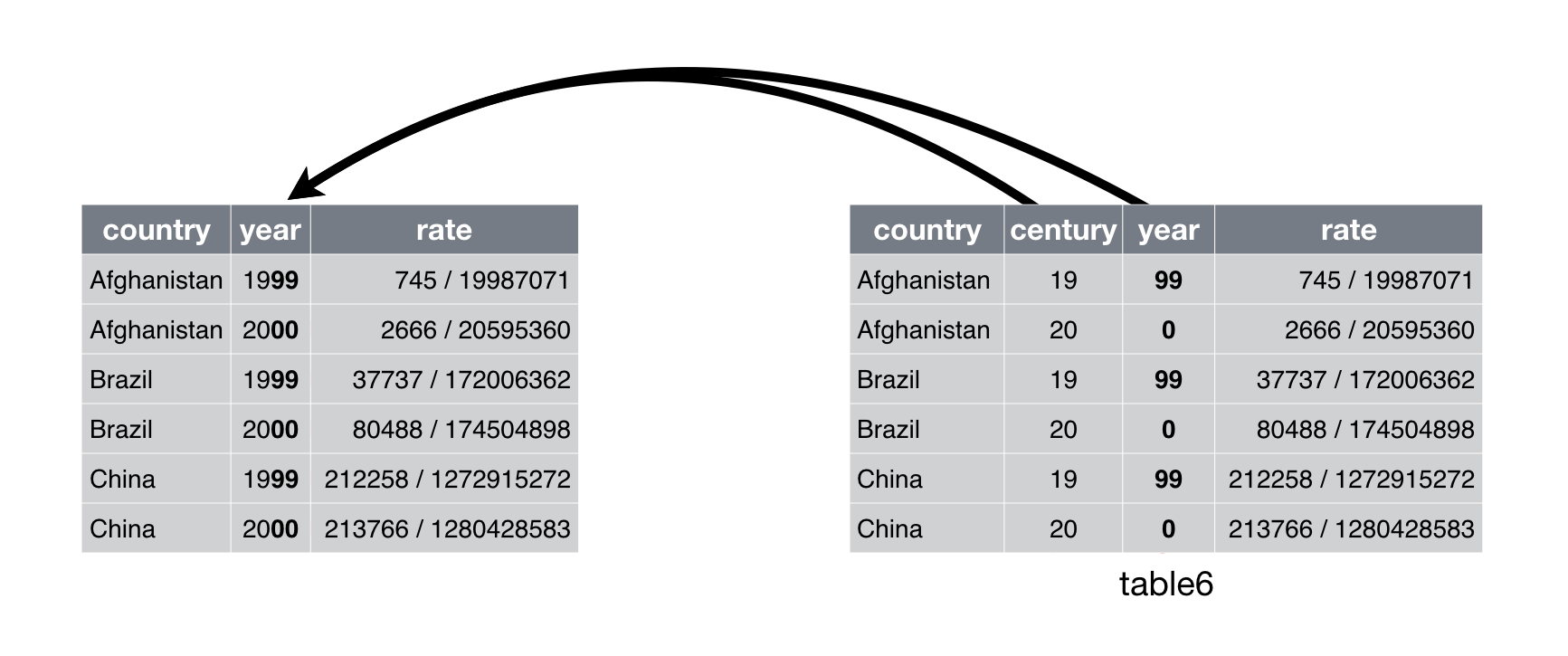
Figure 12.5: Uniting table5 makes it tidy
We can use unite() to rejoin the century and year columns that we created in the last example. That data is saved as tidyr::table5. unite() takes a data frame, the name of the new variable to create, and a set of columns to combine, again specified in dplyr::select() style:
table5 %>%
  unite(new, century, year)
#> # A tibble: 6 × 3
#>       country   new              rate
#> *       <chr> <chr>             <chr>
#> 1 Afghanistan 19_99      745/19987071
#> 2 Afghanistan 20_00     2666/20595360
#> 3      Brazil 19_99   37737/172006362
#> 4      Brazil 20_00   80488/174504898
#> 5       China 19_99 212258/1272915272
#> 6       China 20_00 213766/1280428583
In this case we also need to use the sep argument. The default will place an underscore (_) between the values from different columns. Here we don’t want any separator so we use "":
table5 %>%
  unite(new, century, year, sep = "")
#> # A tibble: 6 × 3
#>       country   new              rate
#> *       <chr> <chr>             <chr>
#> 1 Afghanistan  1999      745/19987071
#> 2 Afghanistan  2000     2666/20595360
#> 3      Brazil  1999   37737/172006362
#> 4      Brazil  2000   80488/174504898
#> 5       China  1999 212258/1272915272
#> 6       China  2000 213766/1280428583
12.4.3 Exercises
What do the
extraandfillarguments do inseparate()? Experiment with the various options for the following two toy datasets.tibble(x = c("a,b,c", "d,e,f,g", "h,i,j")) %>% separate(x, c("one", "two", "three")) tibble(x = c("a,b,c", "d,e", "f,g,i")) %>% separate(x, c("one", "two", "three"))Both
unite()andseparate()have aremoveargument. What does it do? Why would you set it toFALSE?Compare and contrast
separate()andextract(). Why are there three variations of separation (by position, by separator, and with groups), but only one unite?
12.5 Missing values
Changing the representation of a dataset brings up an important subtlety of missing values. Surprisingly, a value can be missing in one of two possible ways:
- Explicitly, i.e. flagged with
NA. - Implicitly, i.e. simply not present in the data.
Let’s illustrate this idea with a very simple data set:
stocks <- tibble(
  year   = c(2015, 2015, 2015, 2015, 2016, 2016, 2016),
  qtr    = c(   1,    2,    3,    4,    2,    3,    4),
  return = c(1.88, 0.59, 0.35,   NA, 0.92, 0.17, 2.66)
)
There are two missing values in this dataset:
The return for the fourth quarter of 2015 is explicitly missing, because the cell where its value should be instead contains
NA.The return for the first quarter of 2016 is implicitly missing, because it simply does not appear in the dataset.
One way to think about the difference is with this Zen-like koan: An explicit missing value is the presence of an absence; an implicit missing value is the absence of a presence.
The way that a dataset is represented can make implicit values explicit. For example, we can make the implicit missing value explicit by putting years in the columns:
stocks %>%
  spread(year, return)
#> # A tibble: 4 × 3
#>     qtr `2015` `2016`
#> * <dbl>  <dbl>  <dbl>
#> 1     1   1.88     NA
#> 2     2   0.59   0.92
#> 3     3   0.35   0.17
#> 4     4     NA   2.66
Because these explicit missing values may not be important in other representations of the data, you can set na.rm = TRUE in gather() to turn explicit missing values implicit:
stocks %>%
  spread(year, return) %>%
  gather(year, return, `2015`:`2016`, na.rm = TRUE)
#> # A tibble: 6 × 3
#>     qtr  year return
#> * <dbl> <chr>  <dbl>
#> 1     1  2015   1.88
#> 2     2  2015   0.59
#> 3     3  2015   0.35
#> 4     2  2016   0.92
#> 5     3  2016   0.17
#> 6     4  2016   2.66
Another important tool for making missing values explicit in tidy data is complete():
stocks %>%
  complete(year, qtr)
#> # A tibble: 8 × 3
#>    year   qtr return
#>   <dbl> <dbl>  <dbl>
#> 1  2015     1   1.88
#> 2  2015     2   0.59
#> 3  2015     3   0.35
#> 4  2015     4     NA
#> 5  2016     1     NA
#> 6  2016     2   0.92
#> # ... with 2 more rows
complete() takes a set of columns, and finds all unique combinations. It then ensures the original dataset contains all those values, filling in explicit NAs where necessary.
There’s one other important tool that you should know for working with missing values. Sometimes when a data source has primarily been used for data entry, missing values indicate that the previous value should be carried forward:
treatment <- tribble(
  ~ person,           ~ treatment, ~response,
  "Derrick Whitmore", 1,           7,
  NA,                 2,           10,
  NA,                 3,           9,
  "Katherine Burke",  1,           4
)
You can fill in these missing values with fill(). It takes a set of columns where you want missing values to be replaced by the most recent non-missing value (sometimes called last observation carried forward).
treatment %>%
  fill(person)
#> # A tibble: 4 × 3
#>             person treatment response
#>              <chr>     <dbl>    <dbl>
#> 1 Derrick Whitmore         1        7
#> 2 Derrick Whitmore         2       10
#> 3 Derrick Whitmore         3        9
#> 4  Katherine Burke         1        4
12.5.1 Exercises
Compare and contrast the
fillarguments tospread()andcomplete().What does the direction argument to
fill()do?
12.6 Case Study
To finish off the chapter, let’s pull together everything you’ve learned to tackle a realistic data tidying problem. The tidyr::who dataset contains tuberculosis (TB) cases broken down by year, country, age, gender, and diagnosis method. The data comes from the 2014 World Health Organization Global Tuberculosis Report, available at http://www.who.int/tb/country/data/download/en/.
There’s a wealth of epidemiological information in this dataset, but it’s challenging to work with the data in the form that it’s provided:
who
#> # A tibble: 7,240 × 60
#>       country  iso2  iso3  year new_sp_m014 new_sp_m1524 new_sp_m2534
#>         <chr> <chr> <chr> <int>       <int>        <int>        <int>
#> 1 Afghanistan    AF   AFG  1980          NA           NA           NA
#> 2 Afghanistan    AF   AFG  1981          NA           NA           NA
#> 3 Afghanistan    AF   AFG  1982          NA           NA           NA
#> 4 Afghanistan    AF   AFG  1983          NA           NA           NA
#> 5 Afghanistan    AF   AFG  1984          NA           NA           NA
#> 6 Afghanistan    AF   AFG  1985          NA           NA           NA
#> # ... with 7,234 more rows, and 53 more variables: new_sp_m3544 <int>,
#> #   new_sp_m4554 <int>, new_sp_m5564 <int>, new_sp_m65 <int>,
#> #   new_sp_f014 <int>, new_sp_f1524 <int>, new_sp_f2534 <int>,
#> #   new_sp_f3544 <int>, new_sp_f4554 <int>, new_sp_f5564 <int>,
#> #   new_sp_f65 <int>, new_sn_m014 <int>, new_sn_m1524 <int>,
#> #   new_sn_m2534 <int>, new_sn_m3544 <int>, new_sn_m4554 <int>,
#> #   new_sn_m5564 <int>, new_sn_m65 <int>, new_sn_f014 <int>,
#> #   new_sn_f1524 <int>, new_sn_f2534 <int>, new_sn_f3544 <int>,
#> #   new_sn_f4554 <int>, new_sn_f5564 <int>, new_sn_f65 <int>,
#> #   new_ep_m014 <int>, new_ep_m1524 <int>, new_ep_m2534 <int>,
#> #   new_ep_m3544 <int>, new_ep_m4554 <int>, new_ep_m5564 <int>,
#> #   new_ep_m65 <int>, new_ep_f014 <int>, new_ep_f1524 <int>,
#> #   new_ep_f2534 <int>, new_ep_f3544 <int>, new_ep_f4554 <int>,
#> #   new_ep_f5564 <int>, new_ep_f65 <int>, newrel_m014 <int>,
#> #   newrel_m1524 <int>, newrel_m2534 <int>, newrel_m3544 <int>,
#> #   newrel_m4554 <int>, newrel_m5564 <int>, newrel_m65 <int>,
#> #   newrel_f014 <int>, newrel_f1524 <int>, newrel_f2534 <int>,
#> #   newrel_f3544 <int>, newrel_f4554 <int>, newrel_f5564 <int>,
#> #   newrel_f65 <int>
This is a very typical real-life example dataset. It contains redundant columns, odd variable codes, and many missing values. In short, who is messy, and we’ll need multiple steps to tidy it. Like dplyr, tidyr is designed so that each function does one thing well. That means in real-life situations you’ll usually need to string together multiple verbs into a pipeline.
The best place to start is almost always to gather together the columns that are not variables. Let’s have a look at what we’ve got:
It looks like
country,iso2, andiso3are three variables that redundantly specify the country.yearis clearly also a variable.We don’t know what all the other columns are yet, but given the structure in the variable names (e.g.
new_sp_m014,new_ep_m014,new_ep_f014) these are likely to be values, not variables.
So we need to gather together all the columns from new_sp_m014 to newrel_f65. We don’t know what those values represent yet, so we’ll give them the generic name "key". We know the cells represent the count of cases, so we’ll use the variable cases. There are a lot of missing values in the current representation, so for now we’ll use na.rm just so we can focus on the values that are present.
who1 <- who %>%
  gather(new_sp_m014:newrel_f65, key = "key", value = "cases", na.rm = TRUE)
who1
#> # A tibble: 76,046 × 6
#>       country  iso2  iso3  year         key cases
#> *       <chr> <chr> <chr> <int>       <chr> <int>
#> 1 Afghanistan    AF   AFG  1997 new_sp_m014     0
#> 2 Afghanistan    AF   AFG  1998 new_sp_m014    30
#> 3 Afghanistan    AF   AFG  1999 new_sp_m014     8
#> 4 Afghanistan    AF   AFG  2000 new_sp_m014    52
#> 5 Afghanistan    AF   AFG  2001 new_sp_m014   129
#> 6 Afghanistan    AF   AFG  2002 new_sp_m014    90
#> # ... with 7.604e+04 more rows
We can get some hint of the structure of the values in the new key column by counting them:
who1 %>%
  count(key)
#> # A tibble: 56 × 2
#>            key     n
#>          <chr> <int>
#> 1  new_ep_f014  1032
#> 2 new_ep_f1524  1021
#> 3 new_ep_f2534  1021
#> 4 new_ep_f3544  1021
#> 5 new_ep_f4554  1017
#> 6 new_ep_f5564  1017
#> # ... with 50 more rows
You might be able to parse this out by yourself with a little thought and some experimentation, but luckily we have the data dictionary handy. It tells us:
The first three letters of each column denote whether the column contains new or old cases of TB. In this dataset, each column contains new cases.
The next two letters describe the type of TB:
relstands for cases of relapseepstands for cases of extrapulmonary TBsnstands for cases of pulmonary TB that could not be diagnosed by a pulmonary smear (smear negative)spstands for cases of pulmonary TB that could be diagnosed be a pulmonary smear (smear positive)
The sixth letter gives the sex of TB patients. The dataset groups cases by males (
m) and females (f).The remaining numbers gives the age group. The dataset groups cases into seven age groups:
014= 0 – 14 years old1524= 15 – 24 years old2534= 25 – 34 years old3544= 35 – 44 years old4554= 45 – 54 years old5564= 55 – 64 years old65= 65 or older
We need to make a minor fix to the format of the column names: unfortunately the names are slightly inconsistent because instead of new_rel we have newrel (it’s hard to spot this here but if you don’t fix it we’ll get errors in subsequent steps). You’ll learn about str_replace() in strings, but the basic idea is pretty simple: replace the characters “newrel” with “new_rel”. This makes all variable names consistent.
who2 <- who1 %>%
  mutate(key = stringr::str_replace(key, "newrel", "new_rel"))
who2
#> # A tibble: 76,046 × 6
#>       country  iso2  iso3  year         key cases
#>         <chr> <chr> <chr> <int>       <chr> <int>
#> 1 Afghanistan    AF   AFG  1997 new_sp_m014     0
#> 2 Afghanistan    AF   AFG  1998 new_sp_m014    30
#> 3 Afghanistan    AF   AFG  1999 new_sp_m014     8
#> 4 Afghanistan    AF   AFG  2000 new_sp_m014    52
#> 5 Afghanistan    AF   AFG  2001 new_sp_m014   129
#> 6 Afghanistan    AF   AFG  2002 new_sp_m014    90
#> # ... with 7.604e+04 more rows
We can separate the values in each code with two passes of separate(). The first pass will split the codes at each underscore.
who3 <- who2 %>%
  separate(key, c("new", "type", "sexage"), sep = "_")
who3
#> # A tibble: 76,046 × 8
#>       country  iso2  iso3  year   new  type sexage cases
#> *       <chr> <chr> <chr> <int> <chr> <chr>  <chr> <int>
#> 1 Afghanistan    AF   AFG  1997   new    sp   m014     0
#> 2 Afghanistan    AF   AFG  1998   new    sp   m014    30
#> 3 Afghanistan    AF   AFG  1999   new    sp   m014     8
#> 4 Afghanistan    AF   AFG  2000   new    sp   m014    52
#> 5 Afghanistan    AF   AFG  2001   new    sp   m014   129
#> 6 Afghanistan    AF   AFG  2002   new    sp   m014    90
#> # ... with 7.604e+04 more rows
Then we might as well drop the new column because it’s constant in this dataset. While we’re dropping columns, let’s also drop iso2 and iso3 since they’re redundant.
who3 %>%
  count(new)
#> # A tibble: 1 × 2
#>     new     n
#>   <chr> <int>
#> 1   new 76046
who4 <- who3 %>%
  select(-new, -iso2, -iso3)
Next we’ll separate sexage into sex and age by splitting after the first character:
who5 <- who4 %>%
  separate(sexage, c("sex", "age"), sep = 1)
who5
#> # A tibble: 76,046 × 6
#>       country  year  type   sex   age cases
#> *       <chr> <int> <chr> <chr> <chr> <int>
#> 1 Afghanistan  1997    sp     m   014     0
#> 2 Afghanistan  1998    sp     m   014    30
#> 3 Afghanistan  1999    sp     m   014     8
#> 4 Afghanistan  2000    sp     m   014    52
#> 5 Afghanistan  2001    sp     m   014   129
#> 6 Afghanistan  2002    sp     m   014    90
#> # ... with 7.604e+04 more rows
The who dataset is now tidy!
I’ve shown you the code a piece at a time, assigning each interim result to a new variable. This typically isn’t how you’d work interactively. Instead, you’d gradually build up a complex pipe:
who %>%
  gather(code, value, new_sp_m014:newrel_f65, na.rm = TRUE) %>%
  mutate(code = stringr::str_replace(code, "newrel", "new_rel")) %>%
  separate(code, c("new", "var", "sexage")) %>%
  select(-new, -iso2, -iso3) %>%
  separate(sexage, c("sex", "age"), sep = 1)
12.6.1 Exercises
In this case study I set
na.rm = TRUEjust to make it easier to check that we had the correct values. Is this reasonable? Think about how missing values are represented in this dataset. Are there implicit missing values? What’s the difference between anNAand zero?What happens if you neglect the
mutate()step? (mutate(key = stringr::str_replace(key, "newrel", "new_rel")))I claimed that
iso2andiso3were redundant withcountry. Confirm this claim.For each country, year, and sex compute the total number of cases of TB. Make an informative visualisation of the data.
12.7 Non-tidy data
Before we continue on to other topics, it’s worth talking briefly about non-tidy data. Earlier in the chapter, I used the pejorative term “messy” to refer to non-tidy data. That’s an oversimplification: there are lots of useful and well-founded data structures that are not tidy data. There are two main reasons to use other data structures:
Alternative representations may have substantial performance or space advantages.
Specialised fields have evolved their own conventions for storing data that may be quite different to the conventions of tidy data.
Either of these reasons means you’ll need something other than a tibble (or data frame). If your data does fit naturally into a rectangular structure composed of observations and variables, I think tidy data should be your default choice. But there are good reasons to use other structures; tidy data is not the only way.
If you’d like to learn more about non-tidy data, I’d highly recommend this thoughtful blog post by Jeff Leek: http://simplystatistics.org/2016/02/17/non-tidy-data/