Chapter 1 R
1.1 General code
1.1.1 检查数据框每列值的分类
df <- read.delim("data/dataCategory_Input.txt")

aofactor <- c("VariantsGroup","GenomeType","Continent","Part_Continent","Subspecies","TreeValidatedGroupbySubspecies","Subgenome","DelCountGroup")

# dfcount <- df %>% summarise(across(.cols = aofactor,.fns = n_distinct))
### 统计每种分类下的因子分别是什么
l <- list() ### 先建立list
for(i in aofactor){
  d <- df[,i]
  d <- d[!is.na(d)]
  l[[i]] <- levels(as.factor(d))
}

fp <- paste("~/Documents/TaxaCategory",".txt",sep="") ### txt format
# fp <- paste("~/Documents/TaxaCategory",".csv",sep="") ### csv format
capture.output(l,file = fp)
1.2 ggplot
1.2.1 geom_text
dftotal <- read.delim("data/geom_text.txt")
aobins <- c(0,0.0385,0.0759,0.113,0.151,0.188,0.225,0.262,0.3,0.45,0.6,0.7,0.8,0.9,1)
vector <-  c(1:length(aobins))[-length(aobins)]
xlabels <- NULL
for (i in vector) {
  print(paste(paste(aobins[i]*100,"%",sep = ""),paste(aobins[i+1]*100,"%",sep = ""),sep = "-") )
  label <- paste(paste(aobins[i]*100,"%",sep = ""),paste(aobins[i+1]*100,"%",sep = ""),sep = "-")
  xlabels[i] = label
}
## [1] "0%-3.85%"
## [1] "3.85%-7.59%"
## [1] "7.59%-11.3%"
## [1] "11.3%-15.1%"
## [1] "15.1%-18.8%"
## [1] "18.8%-22.5%"
## [1] "22.5%-26.2%"
## [1] "26.2%-30%"
## [1] "30%-45%"
## [1] "45%-60%"
## [1] "60%-70%"
## [1] "70%-80%"
## [1] "80%-90%"
## [1] "90%-100%"dfori <- dftotal %>% filter(Region=="CDS",Variant_type=="SYNONYMOUS"|Variant_type=="NONSYNONYMOUS") %>%
mutate(Derived_SIFT = ifelse(is.na(Derived_SIFT),100,Derived_SIFT)) %>%
mutate(Gerp = ifelse(is.na(Gerp),-100,Gerp)) %>%
mutate(LoadGroup = ifelse(Variant_type=="NONSYNONYMOUS",ifelse(Derived_SIFT<=0.05&Gerp>=1,"Deleterious","Nonsynonymous"),"Synonymous")) %>%
filter(!Ancestral == "NA") %>%
filter(Ancestral==Ref|Ancestral==Alt) %>%
mutate(IfRefisAnc = if_else(Ref == Ancestral,"Anc","Der"))
dffre <- dfori %>%
filter(!is.na(DAF_ABD)) %>% ## 注意要保持和分bin后一致,所以这里也要去除 DAF_ABD是NA的值。
group_by(Sub,IfRefisAnc) %>%
count(LoadGroup) %>%
mutate(fre=n/sum(n)) %>%
arrange(Sub,desc(LoadGroup)) %>%
filter(Sub=="A",LoadGroup=="Deleterious")
### data deal
df <- dfori %>%
filter(!is.na(DAF_ABD)) %>%
mutate(bin=cut(DAF_ABD,breaks=aobins)) %>%
group_by(Sub,IfRefisAnc,bin) %>%
count(LoadGroup) %>%
mutate(fre=n/sum(n)) %>%
arrange(Sub,desc(bin)) %>%
### merge group
mutate(group = paste(IfRefisAnc,"-",str_sub(LoadGroup,1,3),sep = ""))
p <- df %>%
filter(Sub=="A") %>%
filter(LoadGroup=="Deleterious") %>%
ggplot()+
geom_line(aes(x=bin,y=fre,group=group,color=group,linetype=group),color = "#d5311c")+
scale_linetype_manual(values=c("solid","dotdash"))+
labs(y="Fraction in each category",x="Derived allele frequency bins")+
# scale_color_brewer(palette = "Set2")+
scale_x_discrete(label = xlabels)+
geom_hline(yintercept = dffre$fre[1],color ="#d5311c")+
# geom_text(aes(0,dffre$fre[1],label = dffre$fre[1], vjust = -1))+
geom_hline(yintercept = dffre$fre[2],color ="#d5311c",linetype="dashed")+
# geom_text(aes(0,dffre$fre[2],label = dffre$fre[1], vjust = -1))+
geom_text(data=dffre,aes(x=1,y=fre,label=round(fre,3)),nudge_y = .01)+
facet_grid(Sub~.)+
theme_classic()+
theme(legend.position = "none")+
theme(axis.text.x= element_text(angle=45, vjust=1,hjust = 1))+
theme(plot.margin=unit(rep(1,4),'lines'),
axis.line = element_line(size=0.4, colour = "black"),text = element_text(size = 10))
p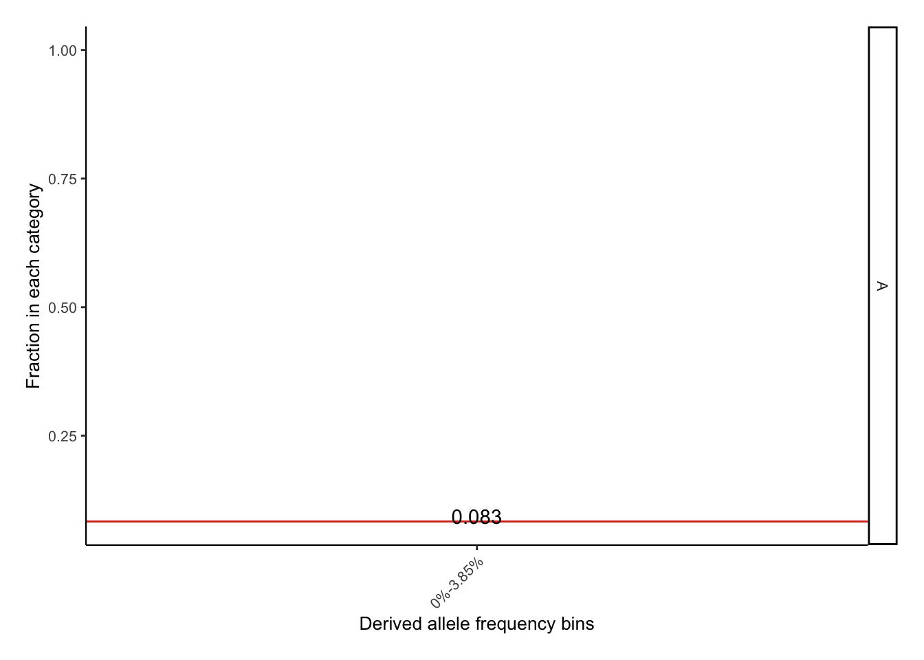
ggsave(p,filename = "~/Documents/test.pdf",height = 9/2.5,width = 16/2.5 )1.3 Strings
mutate(qseqid = str_split_fixed(qseqid, fixed(":"), n=3)[,1]) %>% 1.4 bedtoolsr
library(bedtoolsr)
dataFile <- c("Data/bedtoolsr/query.txt")
df <- read.table(dataFile,sep = "\t",header = T)

dataFile <- c("Data/bedtoolsr/cds.txt")
dfdb <- read.table(dataFile,sep = "\t",header = T)

### 目的:保留选择区和基因库的交集,并且得到交集所在的基因
dfh1 <- bt.intersect(df,dfdb)
dfh2 <- bt.intersect(df,dfdb,wo=dfdb)
dfh3 <- bt.intersect(df,dfdb,wo=df)
dfh4 <- bt.intersect(df,dfdb,wb=dfdb)
dfh5 <- bt.intersect(df,dfdb,wb=df)
dfh6 <- bt.intersect(df,dfdb,wa=dfdb)
dfh7 <- bt.intersect(df,dfdb,wa=df)
dfh8 <- bt.intersect(df,dfdb,wao =dfdb)
dfh9 <- bt.intersect(df,dfdb,wao =df)
dfh10 <- bt.intersect(df,dfdb,loj = dfdb)
dfh11 <- bt.intersect(df,dfdb,loj = df)
dfh12 <- bt.intersect(df,dfdb,v = dfdb)
dfh13 <- bt.intersect(df,dfdb,v = df)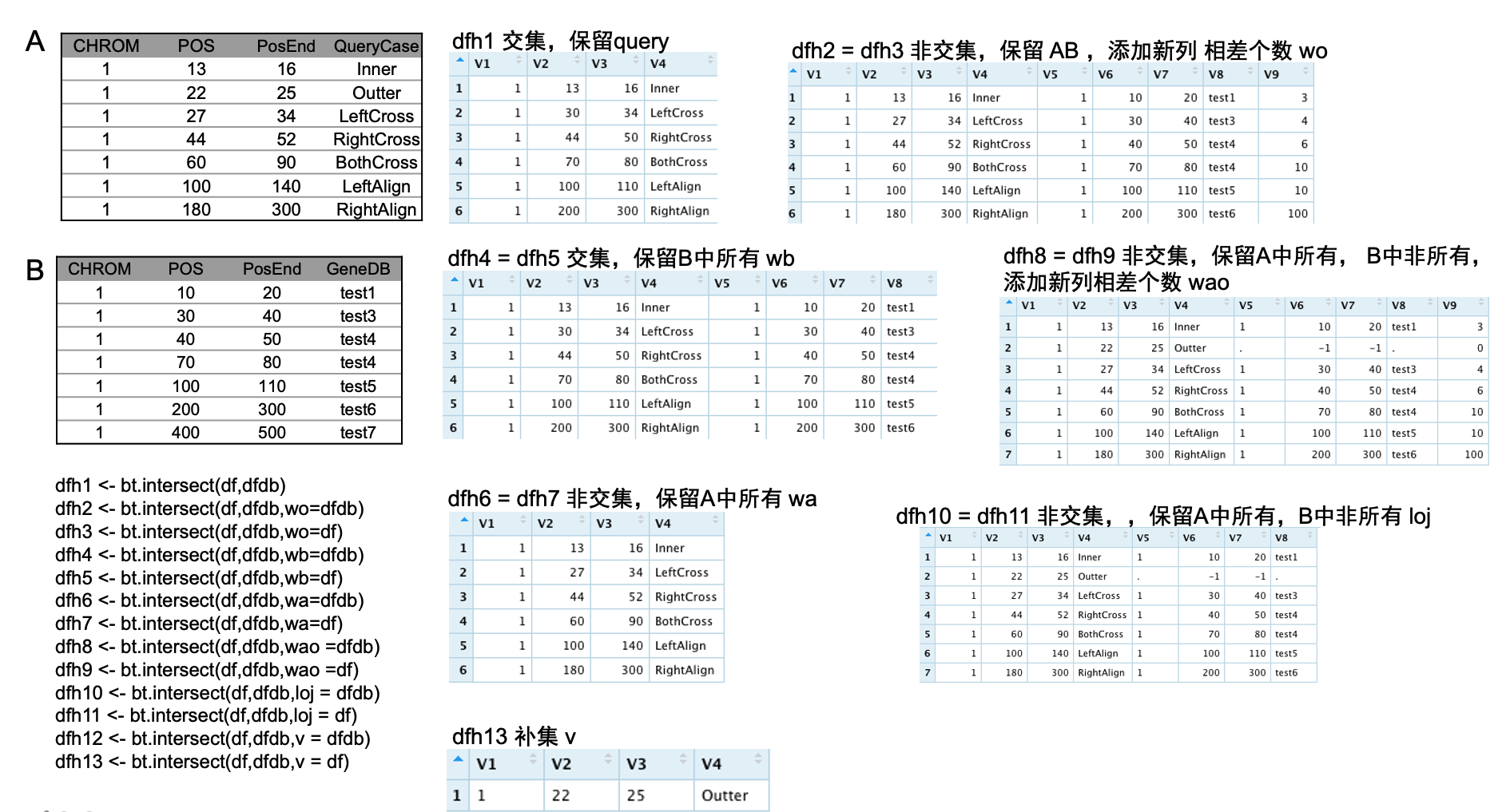
1.5 dplyr
1.5.1 recode
1.6 Plot section
1.6.1 heatmap
############################################################################################################################
### import library and file path
library(tidyverse)
library(pheatmap)
library(RColorBrewer)
infileS <- c("data/001_matrix_pheatmap.txt")
taxaDB <- c("data/001_taxa_InfoDB.txt")
df <- read.delim(infileS,stringsAsFactors = F)
dftaxa <- read.delim(taxaDB,stringsAsFactors = F)
dfinner <- inner_join(data.frame(Taxa=colnames(df)),dftaxa,by="Taxa")
df <- df %>%  select(1:6,all_of(dfinner$Taxa)) ## 选择有亚洲信息的和t

### as matrix
df_num = as.matrix(df[,-1:-6])
# df_num
# df_num[is.na(df_num)] <- 0  ##将缺失值设置为0
# df_num
### 为矩阵添加行名,以行号命名
# rownames(df_num) = paste("row",seq(1,dim(df)[1],1),sep = "")
rownames(df_num) = df$TriadsBlockID
#ncol(df_num)
#nrow(df_num)
### 标准化数据by column
df_num_scale = scale(df_num) ### z = (x — u) / s

### 先画一个最原始的图
# pheatmap(df_num_scale,main = "pheatmap default")
### 去除列上的树
# pheatmap(df_num_scale,cluster_cols = F,main = "pheatmap row cluster")
### 在行上也进行标准化,可以进行行与行之间的比较。注意这里是z score 标准化
# pheatmap(df_num_scale,scale = "row",cluster_cols = T,main = "pheatmap row cluster")

### 建立注释信息数据框,并添加行名
annotation_row = data.frame(rowannotation1 = factor(df$Chr))
# rownames(annotation_row) = paste("row",seq(1,dim(df)[1],1),sep = "") # name matching
rownames(annotation_row) = df$TriadsBlockID
#levels(annotation_row$rowannotation1)
### col annotation data frame
annotation_col=data.frame(colannotation=factor(dfinner$Group))
rownames(annotation_col) =  dfinner$Taxa ######## try

### 自定注释信息的颜色列表
colB <- brewer.pal(9,"Set3")[c(1:7)]
# colC <- c("#fd8582","#ffcbcc","#967bce","#cccdfe","#4bcdc6","#cdfffc","darkgray")
colC <- c("#9900ff","#7B241C","#dbb3ff","#A9A9A9","#fc6e6e","#FF9900","#82C782")
rwb <- colorRampPalette(colors = c("red", "white", "skyblue"))(50)

ann_colors <-  list(colannotation = c(Cultivar=colC[1],LR_Africa=colC[2],
                                                       LR_America=colC[3],LR_CSA=colC[4],
                                                       LR_EA=colC[5],LR_EU=colC[6],
                                                       LR_WA=colC[7]),
                    rowannotation1= c("1A"=colB[1],"2A"=colB[2],"3A"=colB[3],
                                      "4A"=colB[4],"5A"=colB[5],"6A"=colB[6],"7A"=colB[7]))
# ann_colors

### 自定义行名,注意:行名的顺序与原始表格的顺序一致,而不是聚类后的顺序; 也可以显示个别标签
#labels_row = df$TriadsBlockID

# labels_row = c("", "", "", "TP53", "", "", "her2", "", "", "", "", "", "", "", "")
### start to plot !!
p <- pheatmap(
  df_num_scale,
  # df_num,
  # log10(df_num+1) , ## 可以是列标准化的矩阵,也可以是原始矩阵
  scale = "row",
  annotation_row = annotation_row, ## 注释数据框
  annotation_colors = ann_colors, ## 对应注释数据框的因子颜色
  annotation_col = annotation_col,
  annotation_names_row = F,
  annotation_names_col = F,
  main = "",
  cluster_rows = T,
  cluster_cols = T,
  # gaps_row=c(7,14,21,28,35,42),
  # gaps_col=c(3,6,9),
  # cellheight = 8,
  # cellwidth = 8,
  border=FALSE,
  # border_color = "red", border=TRUE,
  show_colnames = F,
  show_rownames = F,
  # labels_row = labels_row,
  # angle_col = "45",
  fontsize = 8, ### all text
  # display_numbers = TRUE,number_color = "blue",number_format = "%.1e" ## display num
  # treeheight_row = 30, treeheight_col = 50 ## tree height,fault 50
  # clustering_method = "average",
  # clustering_distance_rows = "correlation",
  # cutree_rows  = 7, ### Cut the heatmap to pieces
  # cutree_cols = 4, ### Cut the heatmap to pieces
  # gaps_row = c(4, 8),
  color = rwb
  # color = colorRampPalette(brewer.pal(8, "Blues"))(25)
)

#str(p, max.level = 2)
#ggsave(p,filename = "/Users/Aoyue/Documents/heatmap.pdf",height = 7,width = 7)
#ggsave(p,filename = "/Users/Aoyue/Documents/heatmap.png",height = 7,width = 7)
# df_cluster <- df_num[p$tree_row$order, p$tree_col$order]
# write.csv(df_cluster,file="/Users/Aoyue/Documents/value.csv",row.names =T)
1.7 ComplexHeatmap to discrete data
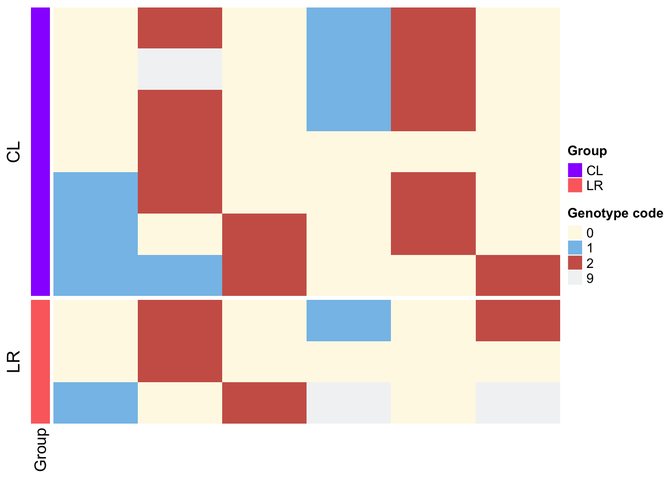
library(ComplexHeatmap)
library(RColorBrewer)
library(circlize) ##加载circlize包,准备为热图设定需要的颜色参数
### 导入数据框,并设置成离散型
df <- read.delim("data/data_forComplexHeatmap.txt") %>%
  arrange(Subspecies) %>%
  pivot_longer(cols = c(X1:X6),names_to = "Col",values_to = "Geno") %>%
  mutate(Geno = as.character(Geno)) %>%
  pivot_wider(names_from = Col,values_from = Geno)

### 转化为矩阵
c1 <- which(colnames(df) == 'Taxa')
c2 <- which(colnames(df) == 'Subspecies')
df_num = as.matrix(df[,-c(c1,c2)])

### 为离散型数据设置颜色
qz <- sort(unique(as.character(df_num)))
colors <- c("#FEF9E7","#85C1E9","#CD6155","#F2F3F4")
names(colors) <- qz
head(colors)
## 0 1 2 9
## "#FEF9E7" "#85C1E9" "#CD6155" "#F2F3F4"### 不保存图片版
Heatmap(df_num,
border = F,
col = colors,name = "Genotype code", ### 设置离散型数据的颜色和图例标题
show_column_names = F,
show_row_names = F,
cluster_rows = F, #cluster_rows:是否列聚类
cluster_columns = F, #cluster_columns:是否列聚类
left_annotation = rowAnnotation(Group =df$Subspecies, col = list(Group = c("LR"="#fc6e6e","CL"="#9900ff"))), ### 设置分组信息的颜色和标题,注意Group 可以改为任何你想改的字符
show_heatmap_legend = T,
row_split = df$Subspecies
)
### 保存图片版
# pdf("~/Documents/test.pdf",height = 4,width = 5)
#
# p <- Heatmap(df_num,
#         border = F,
#         col = colors,name = "Genotype code", ### 设置离散型数据的颜色和图例标题
#         show_column_names = F,
#         show_row_names = F,
#         cluster_rows = F, #cluster_rows:是否列聚类
#         cluster_columns = F, #cluster_columns:是否列聚类
#         left_annotation = rowAnnotation(Group =df$Subspecies, col = list(Group = c("LR"="#fc6e6e","CL"="#9900ff"))), ### 设置分组信息的颜色和标题,注意Group 可以改为任何你想改的字符
#         show_heatmap_legend = T,
#         row_split = df$Subspecies
#         )
#
# draw(p,heatmap_legend_side = "bottom")
# dev.off()
1.7.1 ChIPseeker
1.7.2 ggseqlogo |绘制序列分析图
1.8 Venn
https://rstudio-pubs-static.s3.amazonaws.com/13301_6641d73cfac741a59c0a851feb99e98b.html
https://www.datanovia.com/en/blog/venn-diagram-with-r-or-rstudio-a-million-ways/
1.9 Color
display.brewer.all()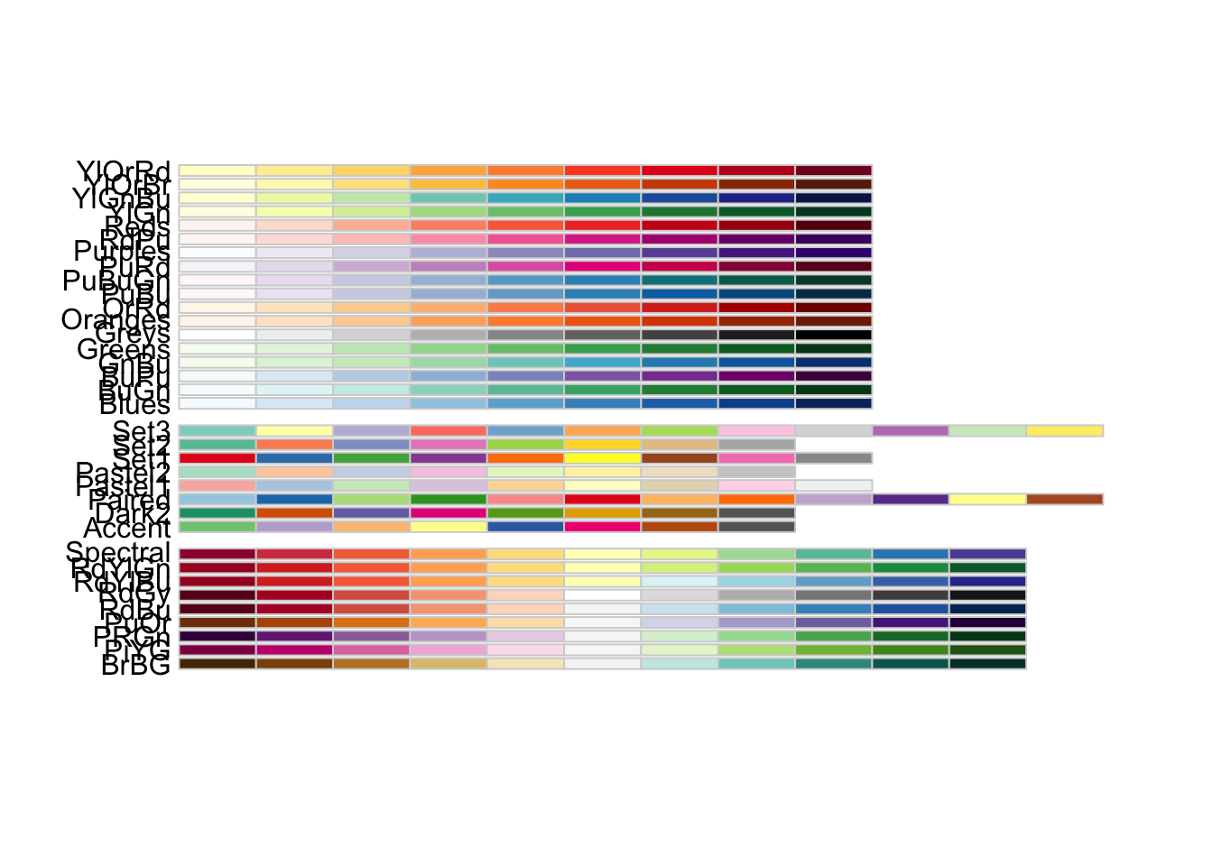
1.10 Trick skills
1.10.1 Pointrange
- point size: fatten
- line size: size
# make test data
df <- data.frame(y=10, ymin=1, ymax=20, x=1)
# store ggplot object
p <- ggplot(data=df, aes(y=y, ymin=ymin, ymax=ymax, x=x))
p + geom_pointrange(fill='blue', color='grey', shape=21, fatten = 10, size = 2)+
  theme_minimal()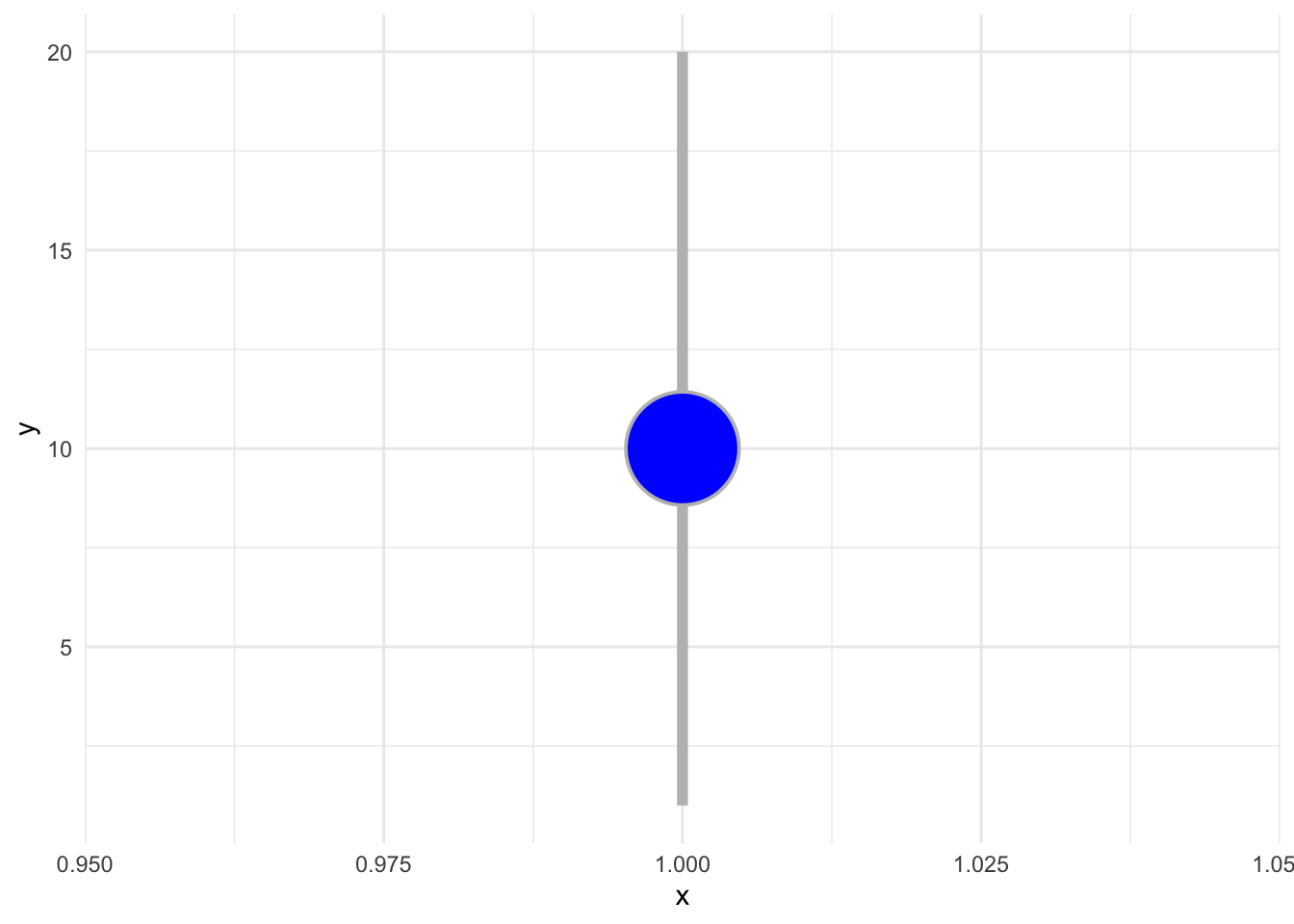
1.10.2 Join 最形象的教程
1.10.3 dplyr trick - %in%
AoSubspecies <- c("EU","CL")
dflrcl <- dfall %>% filter(GroupBySubcontinent %in% AoSubspecies) %>% droplevels()
1.10.4 %>% list -> unset
dfci <- dfeu %>% group_by(SlightlyOrStrongly) %>% summarise(ci=list(mean_cl_normal(T_notEqualVariances))) %>% unnest
1.10.5 custom function in summarise
extractABD <- function(chr){
      library(tidyverse)
      unionChr <- str_c(str_sub(chr[1],5,5),str_sub(chr[2],5,5),str_sub(chr[3],5,5))
      return(unionChr)
    }
    df_filter1 <- df
    df_filter2 <- df %>%
      group_by(qseqid) %>%
      summarise(n=n()) %>%
      left_join(x=df_filter1,y=.,by="qseqid") %>%
      filter(n==3) %>%
      mutate(sub=substring(Chr,5,5)) %>%
      arrange(sub) %>%
      group_by(qseqid) %>%
      summarise(unionChr = extractABD(Chr)) %>%
      left_join(x=df_filter1,y=.,by="qseqid")
1.11 R publish
1.11.1 publish the book
bookdown::publish_book(render = 'local')
1.12 Function
1.12.1 identical : if the two dataframe is equal
identical(a1, a2)
all.equal(a1, a2) #给出哪一列的结果有差别,数值型变量给出均数的相对差异;字符型给出不一致的字符的数目。
match(a1, a2) #NA代表该列不一致 e.g. NA NA 3 (present the first and second column is not equal)
which(a1!=a2, arr.ind = TRUE)
1.12.2 count.fields 统计每行的字段数
`num.fields = count.fields(“combine_test.txt,” sep=“\t”)`\
`num.fields = count.fields(“combine_test.txt,” sep=“\t,”quote = "")`
1.12.3 Merge data and add group
aoaddGroup <- function(infileS,group){
  dfin <- read.delim(infileS)
  dfout <- dfin %>% mutate(DelGroup = group)
  return(dfout)
}

factor1 <- c("003_nonsynGERPandDerivedSIFT","004_nonsynDerivedSIFT","005_GERP","006_nonsynGERPandDerivedSIFT_correction","007_nonsynDerivedSIFT_correction","008_GERP_correction")

inputDir <- c("/Users/Aoyue/project/wheatVMapII/003_dataAnalysis/005_vcf/047_referenceEvaluation/001_delCount_filterLR_CL")
df <- NULL
for (i in factor1) {
  filename <- paste(i,"_additiveDeleterious_ANCbarleyVSsecalePasimony_vmap2_bychr_bySub_delVSsynonymous.txt",sep="")
  infileS <- file.path(inputDir,filename)
  dfo <- aoaddGroup(infileS,i)
  df <- rbind(dfo,df)
}
1.13 Multiple file deal with
inputDir <- c("")
fsList <- list.files(inputDir)
length(fsList)
dfout <- NULL
for (i in fsList) {
  filename <- str_replace(i,".txt","")
  df <- read.table(file.path(inputDir,i),header = T,sep="\t",row.names = NULL)
  df <- df %>% mutate(Subspecies = filename)
  dfout <- rbind(dfout,df)
}

inputDir <- c("")
outputDir <- c("data/001_popDepthBP/")
fsList <- list.files(inputDir)
length(fsList)
for (i in fsList) {
  df <- read.table(file.path(inputDir,i),header = T,sep = "\t",row.names = NULL)
  outfileS <- file.path(outputDir,str_replace(i,".txt.gz",".txt"))

  dfout <- df %>% select(1:16,21)
  write.table(dfout,file=outfileS,quote=F,col.name=T,row.names=F,sep = "\t")
  print(paste(nrow(dfout),"        ", i ,sep = "")) ### log
}