Chapter 3 Standardizing Data

library(fluoR)
df <- format_data(GCaMP)

3.1 Reasons to standardize data

There are a few reasons to standardize your data before exploring your data.

1. Signal differs between subjects

Regardless of the specific technologies used, there is almost always differences in signal strength for each subject

2. Signal differs between trials

The strength of recording signal tends to decay over time

3. Utilizing baseline values

Using transformations such as percent change allows you to center the data at an objective value
After centering your trial and post-trial data, the data is interpreted as relative to baseline values
The baseline period is typically assumed to be a “resting” period prior to exposure to the experimental manipulation. This means that using standardization methods (particularly z-scores) also takes baseline deviations into consideration.

3.2 Methods of standardization

A little alteration in how we compute z-scores can make a significant difference.

3.2.1 z-scores

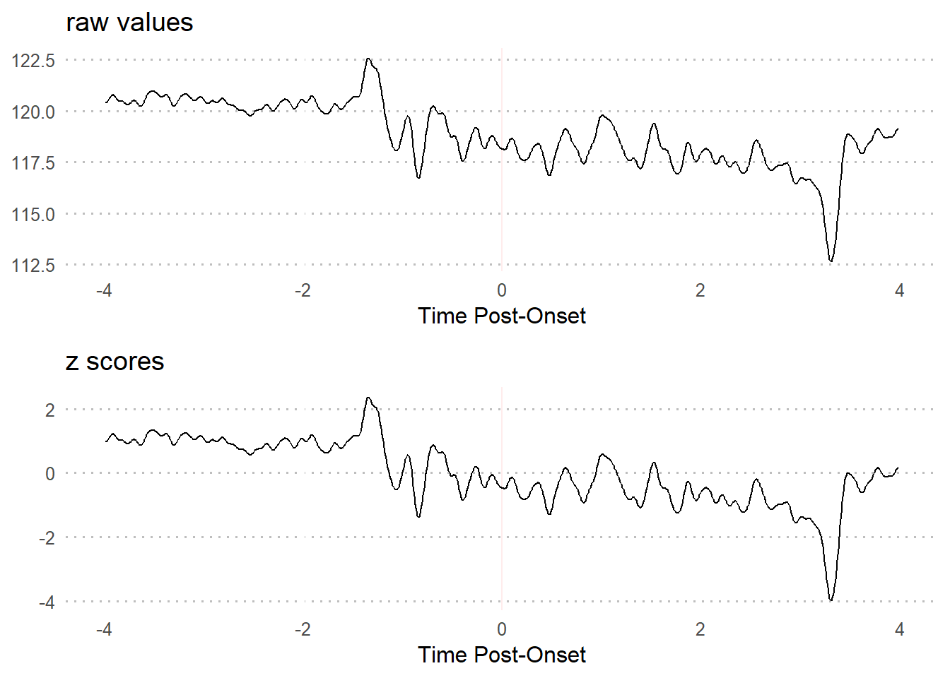
Standard z-score transformations work the same way with time series data as with any other. The formula:

centers every value (x) at the mean of the full time series (mu)
divides it by the standard deviation of the full time series (sigma).

$\begin{gather*} z_{i} = \frac{x_{i}-\mu}{\sigma} \end{gather*}$ $\begin{align*} \text{where...} \\ \mu &= \text{mean of full trial period,} \\ \sigma &= \text{standard deviation of full trial period} \\ \end{align*}$

This results in the same time series in terms of standard deviations from the mean, all in the context of the full time series.

3.2.1.1 R Code

z.scores <- z_score(xvals = df$Trial8,
                    mu = mean(df$Trial8), # manual input of mu/sigma optional;
                    sigma = sd(df$Trial8)) # used for example purposes

3.2.1.2 Visualization

3.2.2 baseline z-scores

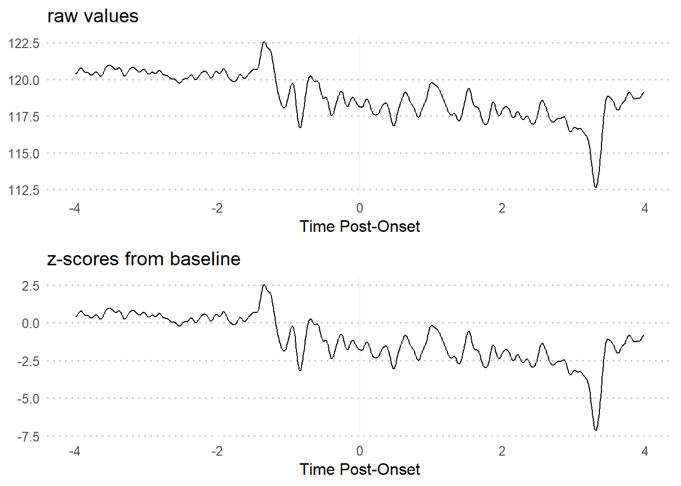
Using the pre-event baseline period as the input values for computing z-scores can be useful in revealing changes in neural activity that you may not find by just comparing pre-trial and trial periods. This is in part because baseline periods tend to have relatively low variability.

As you can see from the formula, a lower standard deviation will increase positive values and decrease negative values - thus making changes in neural activity more apparent.

$\begin{gather*} baseline \ z_{i} = \frac{x_{i}-\bar{x}_{baseline}}{s_{baseline}} \end{gather*}$ $\begin{align*} \text{where...} \\ \bar{x}_{baseline} &= \text{mean of values from baseline period,} \\ {s}_{baseline} &= \text{standard deviation of values from baseline period} \\ \end{align*}$

This results in a time series interpreted in terms of standard deviations and mean during the baseline period. Baseline z-scores are conceptually justifiable because the standard deviation is then the number of deviations from the mean when a subject is at rest. The values outside of the baseline period will be different using this version, but not within the baseline period.

3.2.2.1 R Code

### Extract baseline values
baseline.vals <- df$Trial8[df$Time >= -4 & df$Time <= 0]

### Compute z-scores
z.scores.baseline <- z_score(xvals = df$Trial8,
                             mu = mean(baseline.vals),
                             sigma = sd(baseline.vals))

3.2.2.2 Visualization

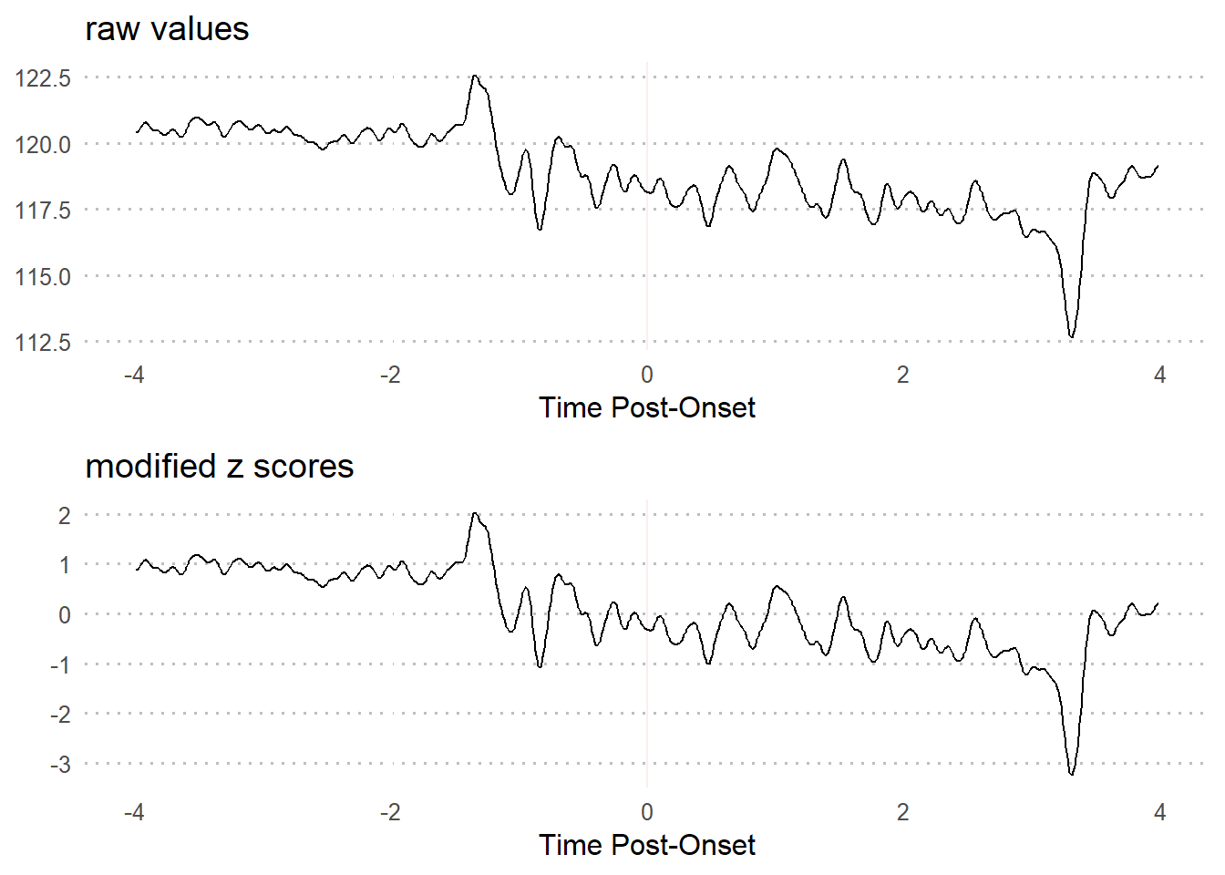
3.2.3 modified z scores

Waveform data fluctuates naturally. But in the event of a change in activity due to external stimuli, signal variation tends to rapidly increase and/or decrease and becomes unruly.

$\begin{gather*} modified \ z_{i} = \frac{0.6745(x_{i}-\widetilde{x})}{MAD} \end{gather*}$ $\begin{align*} \text{where...} \\ \widetilde{x} &= \text{sample median,} \\ {MAD} &= \text{median absolute deviation} \end{align*}$

3.2.3.1 R Code

z.scores.modified <- z_score(xvals = df$Trial8, 
                             z.type = 'modified')

3.2.3.2 Visualization

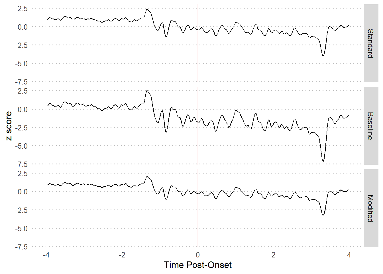
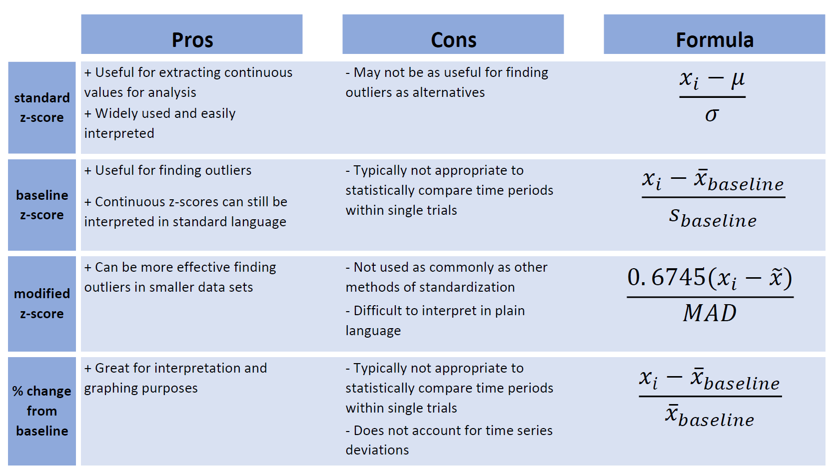
3.3 z-score comparison

3.3.1 Visualization

3.3.2 Summary table

3.4 Examples

3.4.1 Example 1

Standardize trial 8 so that the units are in terms of standard deviations from the mean of the full time series.

z_score(xvals = df$Trial8,
        z.type = 'standard')

3.4.2 Example 2

Standardize trial 8 so that the units are in terms of standard deviations from the mean of the pre-event period.

We can do this manually for each trial.

### Manual
baseline.vals <- df$Trial8[df$Time >= -4 & df$Time <= 0] # extract baseline values
  
baseline.z <- z_score(xvals = df$Trial8,
                      mu = mean(baseline.vals), # mean of baseline
                      sigma = sd(baseline.vals), # sd of baseline
                      z.type = 'standard')

Or we can use the baseline_transform wrapper.

baseline.zdf <- baseline_transform(dataframe = df,
                                   trials = 8,
                                   baseline.times = c(-4, 0),
                                   type = 'z_standard')

Both methods will result in the same values.

all(baseline.zdf$Trial8 - baseline.z == 0)

## [1] TRUE

3.4.3 Example 3

Standardize trial 8 so that the units are in terms of deviations from the median of the full time series.

z_score(xvals = df$Trial8,
        z.type = 'modified')

3.4.4 Example 4

Convert trial 8 so that the units are in terms of percent change from the mean of the pre-event period.

We can do this manually for each trial.

### Manual
baseline.vals <- df$Trial8[df$Time >= -4 & df$Time <= 0] # extract baseline values
  
perc.change <- percent_change(xvals = df$Trial8,
                              base.val = mean(baseline.vals))

Or we can use the baseline_transform wrapper.

perc.changedf <- baseline_transform(dataframe = df,
                                    trials = 8,
                                    baseline.times = c(-4, 0),
                                    type = 'percent_change')

Both methods will result in the same values.

all(perc.changedf$Trial8 - perc.change == 0)

## [1] TRUE